I need to assess the band contribution of different bands of Sentinel 2 and Sentinel 1 to my classified image.
I will really appreciate some help here.
Regards,
Pamela
I need to assess the band contribution of different bands of Sentinel 2 and Sentinel 1 to my classified image.
I will really appreciate some help here.
Regards,
Pamela
If you have classified the image you should know the contribution.
Or you should tell us how you have classified the image and give some more information.
Otherwise we can’t help.
Thanks Marpet. Yes, I have classified the image using Random Forest with very good results. And the legend shows the percentage of the landcover classes for each class. However, I want to see which bands show the best separability for each class. So, for example, for Sentinel 2, does band 4, 5, 6 separate the woody vegetation better than bands 2, 3,8?
I don’t know whether I am making sense.
So this more like a scientific discussion. Finding the best band combination for classification.
So, I’m out, others can chime in.
Thanks:-). Waiting for others…
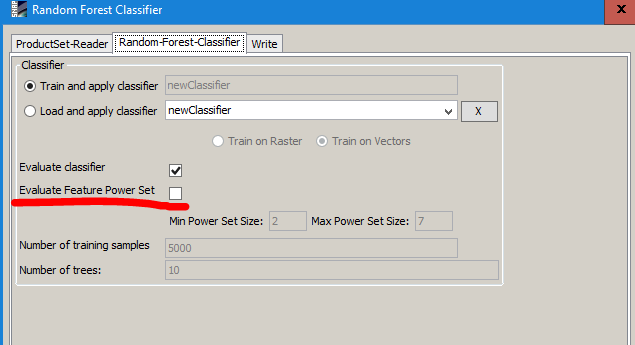
the random forest classifier actually outputs feature importances as well if you check “evaluate feature power set”
A text file should pop up where a % value for each band is given according to its contribution to the RF model.
Great! Let me try this and see what results I will get.
Thanks ABraun.
Regards
Pamela
So I have checked the ‘evaluate power set’ button and the test file has this information at the bottom:
Testing feature importance score:
Each feature is perturbed 3 times and the % correct predictions are averaged
The importance score is the original % correct prediction - average
rank 1 feature 1 : Sigma0_VH_db score: tp=0.5052 accuracy=0.1684 precision=0.6108 correlation=0.5795 errorRate=-0.1684 cost=-Infinity GainRatio = 0.3371
rank 2 feature 2 : Sigma0_VV_db score: tp=0.3618 accuracy=0.1206 precision=0.4530 correlation=0.4528 errorRate=-0.1206 cost=-Infinity GainRatio = 0.3194
Is this the info you were talking about and if so, then how does one interpret this?
that means that S0_VH was more often used than S0_VV. There should be somewhere also a % value besides true positive (tp), accuracy, precision and errorRate.
But as a random forest’s effectiveness strongly relies on perturbation of the input datasets you should use more than just two rasters. Or didn’t you copy the whole feature evaluation?
In this case I was carrying out RF classification on a dual polarised S1 dataset (2 bands, VV and VH). I had about 8 or 9 training classes. Full text report is here:
Cross Validation
Number of classes = 6
class 1.0: Croplandoff
accuracy = 0.9031 precision = 0.2353 correlation = 0.2691 errorRate = 0.0969
TruePositives = 4.0000 FalsePositives = 13.0000 TrueNegatives = 229.0000 FalseNegatives = 12.0000
class 2.0: Croplandon
accuracy = 0.8915 precision = 0.1429 correlation = 0.1687 errorRate = 0.1085
TruePositives = 2.0000 FalsePositives = 12.0000 TrueNegatives = 228.0000 FalseNegatives = 16.0000
class 3.0: Grassland
accuracy = 0.9651 precision = 0.0000 correlation = 0.0176 errorRate = 0.0349
TruePositives = 0.0000 FalsePositives = 4.0000 TrueNegatives = 249.0000 FalseNegatives = 5.0000
class 4.0: Rock
accuracy = 0.8837 precision = 0.6000 correlation = 0.5722 errorRate = 0.1163
TruePositives = 21.0000 FalsePositives = 14.0000 TrueNegatives = 207.0000 FalseNegatives = 16.0000
class 5.0: WB_BS
accuracy = 0.8721 precision = 0.7910 correlation = 0.7167 errorRate = 0.1279
TruePositives = 53.0000 FalsePositives = 14.0000 TrueNegatives = 172.0000 FalseNegatives = 19.0000
class 6.0: Woodyveg
accuracy = 0.9341 precision = 0.8843 correlation = 0.8753 errorRate = 0.0659
TruePositives = 107.0000 FalsePositives = 14.0000 TrueNegatives = 134.0000 FalseNegatives = 3.0000
Using Testing dataset, % correct predictions = 72.4806
Total samples = 519
RMSE = 1.3738984311894407
Bias = 0.08914728682170558
Distribution:
class 0.0: Builtup 1 (0.1923%)
class 1.0: Croplandoff 32 (6.1538%)
class 2.0: Croplandon 36 (6.9231%)
class 3.0: Grassland 11 (2.1154%)
class 4.0: Rock 75 (14.4231%)
class 5.0: WB_BS 144 (27.6923%)
class 6.0: Woodyveg 221 (42.5000%)
Testing feature importance score:
Each feature is perturbed 3 times and the % correct predictions are averaged
The importance score is the original % correct prediction - average
rank 1 feature 1 : Sigma0_VH_db score: tp=0.5052 accuracy=0.1684 precision=0.6108 correlation=0.5795 errorRate=-0.1684 cost=-Infinity GainRatio = 0.3371
rank 2 feature 2 : Sigma0_VV_db score: tp=0.3618 accuracy=0.1206 precision=0.4530 correlation=0.4528 errorRate=-0.1206 cost=-Infinity GainRatio = 0.3194
seems to work (technically) but you can condisder adding image textures (GLCM) as additional input layers so the random forest classifier can really take “random” samples of features and training data.
Thanks. In the final RF classification, I included two seasons of S1 (wet and dry), plus added a S2 image. with this combination, I managed a 96% accuracy.
I would love to know how to add the image textures in SNAP.
yiu find it under Raster > Image analysis > Texture analysis > Grey Level Co-Occurence Matrix. You can simply add them as additional layers for the RF.
Great! I will try this. Many thanks.
Hello,
Is there info on how SNAP is evaluating the power set (method name or reference)? I don’t find that in the help of SNAP.
Thank you
Hello,
I also have the same question.
Hi Pamochungo,
Did you figure out how to evaluate the feature/band importance?
Thanks,
Can I check how long it takes for RF to run when checking “evaluate feature power set”?
I am classifying a subset of approx 25km2 Sentinel-2 image with 12 bands and 5 PCA components and the process seems to take hours. (My machine has 16G RAM in case it matters). I’m new to SNAP so it’s possible my workflow has flaws, any tips would be much appreciated ![]()
Running RF without checking “evaluate feature power set” only takes seconds.