Artefacts in S1TBX radiometric terrain flattening

[eyeinsky]

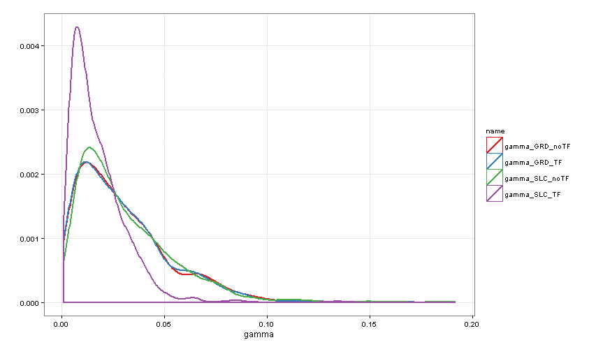
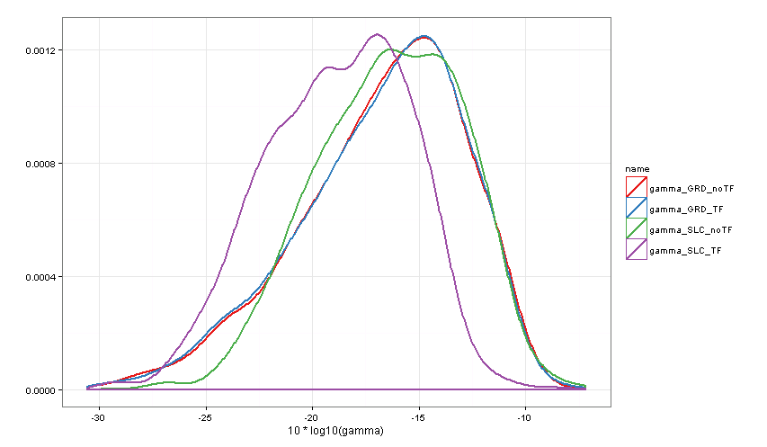
I ran some comparison tests on the S1TBX radiometric terrain flattening, using an IW GRDH image from the region SW of Vienna, Austria. I flattened the backscatter first using my own software using (a) SRTM3, and (b) SRTM1, and compared it with backscatter retrieved after flattening and terrain correction in SNAP (Cal_TF_TC).

It is worth noting the SNAP v2 beta 06 cannot be used for such testing, as the radiometric calibration is off by over 30dB in general. I therefore had to use SNAP v2 beta 05 for the test. SNAP does not support multilooking before terrain flattening, so the flattening was performed on the full resolution image: Cal->TF->TC.

In comparison to the S1TBX result, we noticed the following differences:

1. striping in S1TBX flattened backscatter (at very high zoom levels)

2. very different backscatter in regions with strong slopes: S1TBX often appears to overcompensate on foreslopes and under-“brighten” on backslopes. These are differences of over ±5dB, so very significant

3. an overall trend of a few dB across range, with S1TBX being relatively darker towards far range.

4. The IW2/IW3 subswath boundary, not visible in a simple GTC becomes (faintly) visible in the flattened images. It is due to approximations within the S1IPF still being used when this image was procesed in March 2015. More recent versions of the S1IPF (already being used in production) should be less susceptible to generating such artefacts.

I wondered what terrain-flattening method is implemented in SNAP. The online docs state http://step.esa.int/main/doc/:
SNAP and Sentinel Toolboxes provide integrated help directly from the software itself.

After searching for a while in the software’s help, I noticed a reference to my paper (see above).

This operator removes the radiometric variability associated with topography using the terrain flattening method proposed by Small [1] while leaving the radiometric variability associated with land cover.
Reference:
[1] David Small, “Flattening Gamma: Radiometric Terrain Correction for SAR imagery”, IEEE Transaction on Geoscience and Remote Sensing, Vol. 48, No. 8, August 2011

But given the differences between the results (see below), it would appear that there are large differences between the respective software implementations. That raises the question: what is the algorithm description that best describes what is actually being run in SNAP?

---

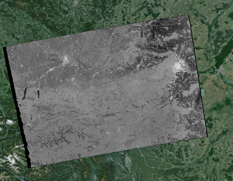
RTC using method of Small, TGRS 2011:

Cal_TF_TC output by SNAP v2 beta 05 (beta 06 not operative for applications requiring radiometric calibration):

---

GTC:

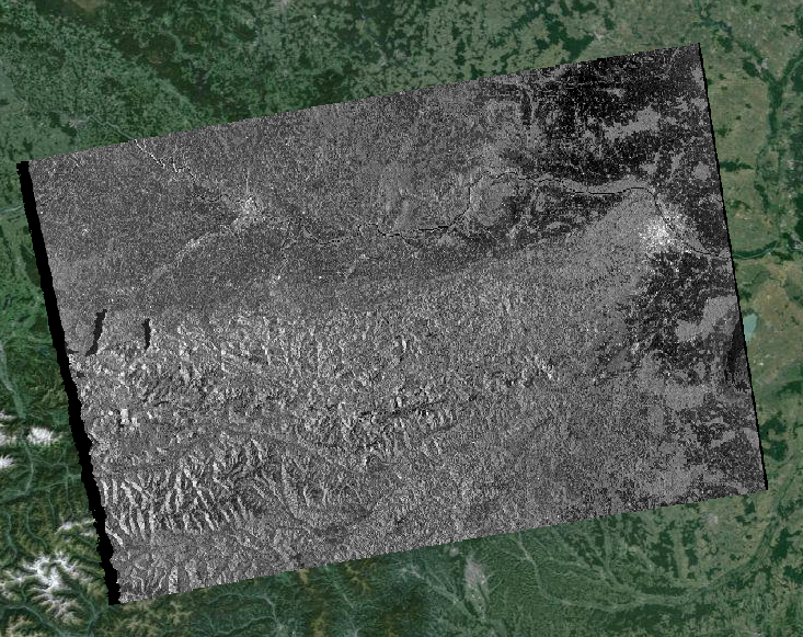
N.B. all 3 images have identical radiometric scales: -26dB (black) to -1dB (white).

[eyeinsky]

Two further points:

A) The post on the striping observed (point 1 above) is here:

Striping after terrain flattening

Hi, Further to the discussion on terrain flattening, I found serious problems with striping in some terrain flattened products. I am running tests with ascending and descending images. Striping occurs in ascending images only (in my set). In particular this scene: S1A_IW_GRDH_1SDV_20150320T165027_20150320T165052_005118_00670A_80F3 (but also the neighbouring one) suffers from striping when running the sequence: Thermal Noise Removal (TNR) -> Calibration -> Terrain Flattening (TF) using…

B) The GTC image is sigma0 ellipsoid backscatter, not gamma0. That explains a slightly different level and trend across range.

[mengdahl]

Thank you for your report David, we’ll look into the issue.

Marcus

[glemoine]

Marcus,

Would it be possible to give an idea when this issue may be resolved? We put some large volume processing activities on hold, in order to avoid reprocessing at a later stage. An alternative is to dig through the code ourselves, but that is definitely non-trivial. On the other hand, this may be an option if resolution still takes considerable time.

Guido

[lferreira]

I built the last code and using an internal DEM or SRTM 3arcsec/1arcsec gave much better results. The striping on the steep hillsides, on the sensor view side, are still there.

[glemoine]

Thanks! I will test the code release in that case. I am not sure the striping is the same as what I have noticed earlier (regular straight striping across range), but that’s something to find out. Your striping sounds less problematic.

Guido

[mengdahl]

It looks like there are still problems with the radiometric terrain flattening in SNAP that the upcoming release will not solve. I hope we can work together with @eyeinsky to find out where our implementation goes wrong.

[clardeux]

About that, because I don’t understand all, I would like to know if the terrain flattening will integrate the correction between sub swath and also due between the different incidence angle ?
Indeed, divided every line by the average of every line works well buts it’s complicated to apply that because all data are not homogeneous.

Best.

[glemoine]

I did a couple of tests with the Beta 8 compiled version. I found that terrain flattening is different from before, but still not the same as what @eyeinsky generates. The cross-range striping is no longer present, even when processing with SRTM 1Sec HGT. The order of steps is still important (e.g. ML -> TF is different from TF -> ML). I can run the full processing chain in one go (Border Noise Removal -> Calibration -> ML -> TF -> TC) and all seems to be a little faster than before.
So, progress, but we’d be very interested if results would converge.

Guido

[clardeux]

Nice news.

However, I don’t know if it’s possible to share beta 8 because I don’t know how to compile it ?

Best

[glemoine]

I understand Beta 8 is to be released this week, before the hackathon at ESRIN (15 & 16 Sept.)

[lferreira]

yep, Luis Veci @lveci also said that on is communication, the next Beta it would be closely released. At min 16.

http://livestream.com/ESA/eoscience/videos/101790018

http://www.eoscience20.org/

About sharing the SNAP build, it’s free open source, just be sure you’ll be sharing the same specs (win/unix, 32bits/64bits)

[lveci]

We’re getting there but it’s still not perfected

[glemoine]

Luis,

As a follow up on the terrain flattening issue, are there plans to correct the procedure so that it is in line with David Small’s algorithm?

Guido

[lveci]

We don’t have plans to revisit this yet.

[Guillaume]

@lveci and @mengdahl : Can you update us on the TF algorithm status?

Does it worth to invest and use it ?

[Guillaume]

Continuing on this topic which might be the main reason to keep SNAP for processing (and not moving to GEE GRD collection).

I tested the impact of two factors on the resulting Gamma0 : 1) starting from SLC or GRD base product 2) with or without TF.

Equivalent source products used :
SLC : S1A_IW_SLC__1SDV_20150821T055817_20150821T055844_007357_00A1B9_4D44.zip
GRD : S1A_IW_GRDH_1SDV_20150821T055818_20150821T055843_007357_00A1B9_0046.zip

I tested 4 processing chains using SRTM 1s (30m) on SNAP v4.0.1 + S1TBX 4.0.0 :

1. <GRD> -> Orbit -> Cal -> Thermal -> TC -> <Gamma_GRD_noTF>
2. <GRD> -> Orbit -> Cal -> Thermal -> TF -> TC -> <Gamma_GRD_TF>
3. <SLC> -> Orbit -> Cal -> Thermal -> TOPSAR-deburst -> Multilook (5x1) -> TC -> <Gamma_SLC_noTF>
4. <SLC> -> Orbit -> Cal -> Thermal -> TOPSAR-deburst -> Multilook (5x1) -> TF -> TC -> <Gamma_SLC_TF>

Here is the resulting Gamma0 VH distributions along a random profile of 10 km across the scene (y in percent) :

or in dB:

The only processing chain showing an effect of the TF is the one starting from SLC product ! In all the other cases, we yield about the same result.

@eyeinsky : David, can you try your test again but starting from a SLC product on SNAP ?

+(It doesn’t look like there is striping any more)

[eyeinsky]

Sorry for the delayed response - I was away on vacation.

That surprises me that SLC vs. GRD should not give consistent results. Can you please specify which version of SNAP you were using?

[Guillaume]

I’m using SNAP v4.0.1 + S1TBX 4.0.0. Thank you for looking at this !

[eyeinsky]

Before TF one should prepare a Cal Beta_Nought, not a Cal Gamma_Nought. That may explain part of the lack of correspondence between the histograms. i.e. one should compare gamma_GRD_noTF with beta_GRD_TF, not with gamma_GRD_TF.