Well, there was Iw2 (5 to 7 bursts)in descending mode processing, but when I want to process ascending mode, my study area falls into two swathes. Do I have to use images of both modes to get vertical changes?
if you want precise ones, yes.
There is a less precise work around presented here: Phase to Displacement Units? - #7 by johngan
Hi There,
I am very impressed by seeing the manual and the codes you have provided, but unfortunately, I am not able to do the same as I don’t have any coding background.
So can you please help me with a video tutorial on how to execute the codes you have mentioned.
This will be of great help as it will help me a lot in doing my master’s thesis.
TIA
have you seen these?
There are also written step-by-step tutorials here:
- https://gitlab.com/Rexthor/gis-blog/-/tree/master/StaMPS
- https://github.com/gjvanleeuwen/SNAP-StaMPS-Visualizing
Actually, you don’t need to be an expert at coding. These scripts are mostly ready to use. The only thing you have to do is to adjust the variables (would be the same in a GUI).
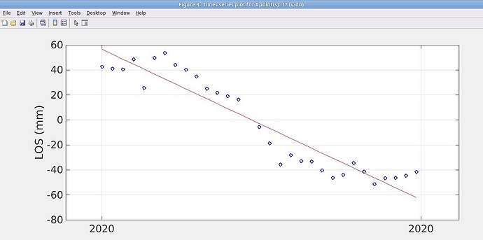
looks great! negative is subsidence, positive is uplift. You can check the quality of the time-series by plotting the displacement for a selected area using the ‘ts’ option. This shows the temporal trend but also the amount of noise in the data.
yes, very good. The screenshot indicates that this trend represents the average displacement of 17 PS.
It shows that they all lay along a clearly negative trend, but with smaller variation. This can be either by an unsteady movement over time (decelerating subsidence in the first half and accelerating in the second half) or by signal noise and atmospheric disturbance. But as all dates agree on the general trend, you can trust that this area is characterized by real subsidence and not just noise within the data. You can repeat this for several points to check if all regions in your study area have this kind of stable trend. Atmospheric outliers will be the same throughout all locations (e.g. the 5th point could be one if it is off the trend in other locations as well).
An example on the interpretation of these time-series is given in the last part of this article: https://www.tandfonline.com/doi/full/10.1080/22797254.2020.1789507
How many ‘ts’ are needed for each part(year)?
the question is how much you need to go sure if the spatial pattern looks trustful.
I do not know the answer to your question because I am really new and inexperienced in this work  . . I intend to get an acceptable output from these processes and submit them for my doctoral dissertation. So far, I have learned from this association. Can you tell me all the codes I need and you in my article that you linked to me? Thank you
Especially when you are less experienced you should not just follow guidelines and trust the result. One crucial aspect for every DInSAR analysis is gaining knowledge on the error sources and getting a feeling about the reliability of the results.
It makes little sense to apply scripts without knowing what they do. In a doctoral dissertation you proof to others that you can develop ideas, understand and apply methods of others, and test hypotheses based on your own analyses.
Have a look at the results - do they make sense? What’s the amount of noise for the different areas. The time-series plot indicates well how noisy the data is. Compared to the time-series of the linked study, your plot looks much more linear and less noisy. If this is the same case for the others, you can start interpreting the results.
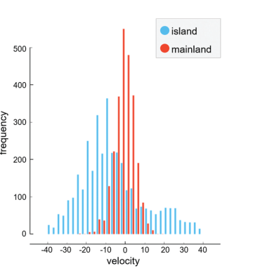
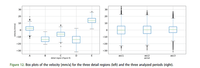
Dear ABraun, thank you very much for your excellent answer. How do I know how low the noise is in similar cases?How can I create the following histograms and Box plots for every part?thanks

I exported the PS as kml file as described in the StaMPS manual, imported them into QGIS and intersected them with polygons, dividing them into island and mainland, and also extracting them from the different locations (A-E). I then exported the intersected points as CSV and created the boxplots in Python.
Can you say me more easily about the S1-TOPSAR-Merge in snap2stamps?
according to this post, snap2stamps currently only supports the processing of one sub-swath.
Hi all.
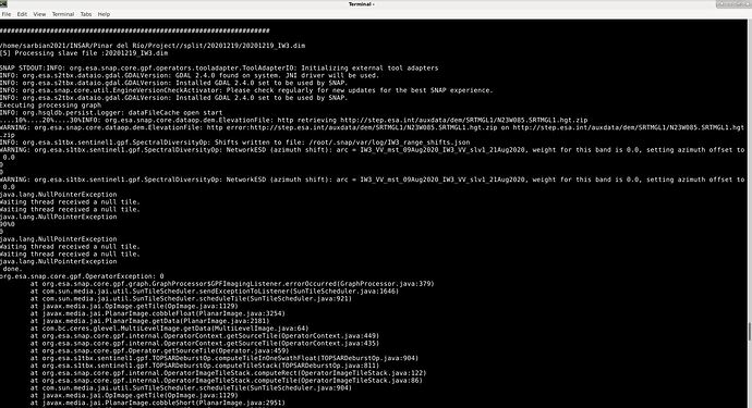
I am getting the following problem when applying the code coreg_ifg_topsar.py
Serco Italia SPA (2020). SNAP2StaMPS: Data preparation for StaMPS PSI processing with SNAP -
Mexico City 2020 (version 1.1). Retrieved from RUS Lectures at https://ruscopernicus.eu/portal/the-rus-library/learn-by-yourself/
I am working on SNAP v. 8.0
Can someone help me, please?
snap2stamps is ready to work with SNAP (v6.0), a bit old, but one day it will be updated.
As you claim to be using SNAP 8, my main question is… had you prepared/modified the needed lines on the coreg_ifg graph used?
Not sure if you get something from SERCO or from the snap2stamps github repository or zenodo package.
More info = more help
Hi @mdelgado, but if I use SNAP 8.0 with snap2stamps from zenodo package what happens?
Thanks.
The ESD operator got an update already in SNAP 7, so the graph xml is slightly different.
I invite you to search in the forum as the solution is somewhere indicated.
Do you refer to UseSuppliedRange/AzimuthShift or also other parms?


