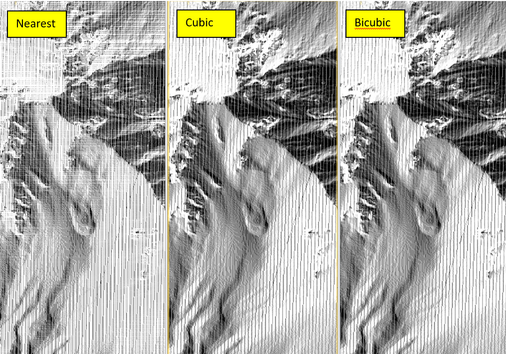
are you sure you changed the DEM Resampling method (first in the image below)? If you select Nearest Neighbor here, the raster should look different.

No worries, I realized that it is the local incidence angle (looks like a hillshade image)
are you sure you changed the DEM Resampling method (first in the image below)? If you select Nearest Neighbor here, the raster should look different.
No worries, I realized that it is the local incidence angle (looks like a hillshade image)
can you please use SRTM 1Sec HGT (AutoDownload) and compare the local incidence angle?
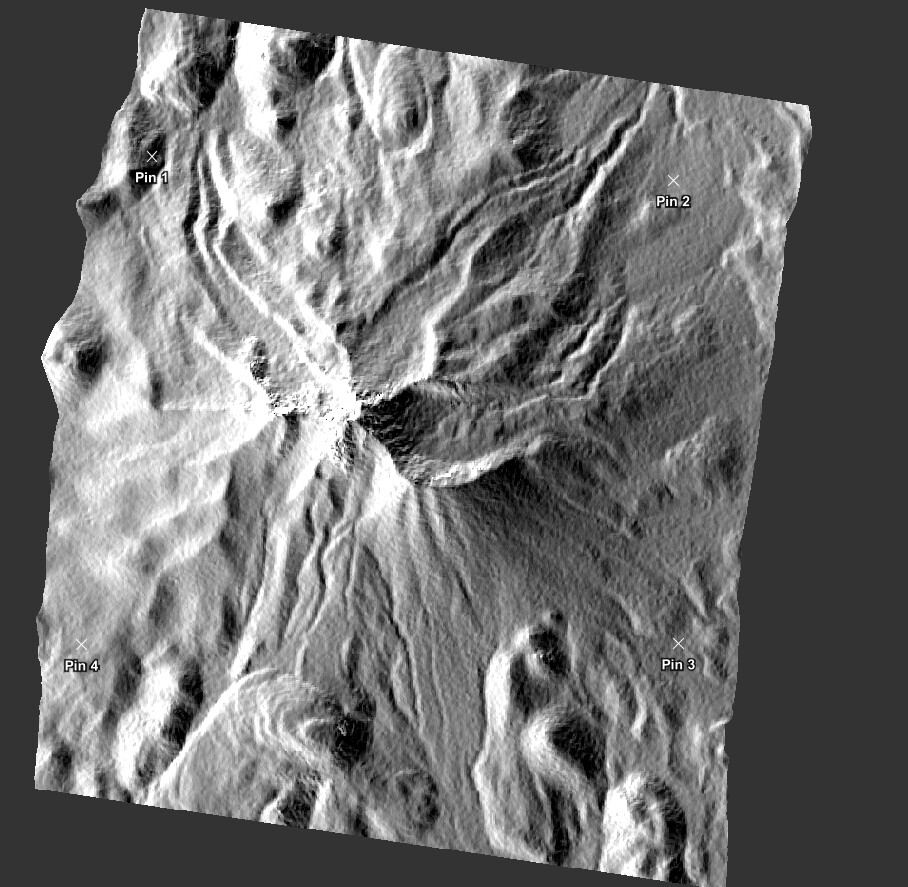
I used SRTM 1Sec HGT (AutoDownload), you right, its normal as you see in image; But I need data which have high spatial resolution for my study. Because I will take local incidence angle values from each pixel for my 1km*1km area.
Is there any chance I could fix this problem occurring with my external DEM?
did you re-project the external DEM to WGS84 before using it in SNAP?
Maybe the stripes were already introduced in this step.You can check by creating a hillshade of the external DEM to see if the stripes are already in the data before using it in SNAP.
Many thanks for your replies. You are right. I controlled my external DEM hillshade and I realized that my data already have stripes. I will look for a solution for this.
Thanks for your time.
Probably also because of the resampling of the DEM?
Hello all,
(@ABraun, @mengdahl, @Zane, @steekhutzie, @tarik44, @gbaier)
I see it’s an old problem, I think I have some news.
Most of those who encountered the stripes phenomena only saw that after processing, and when searching for the problem they tried to process it in different way.
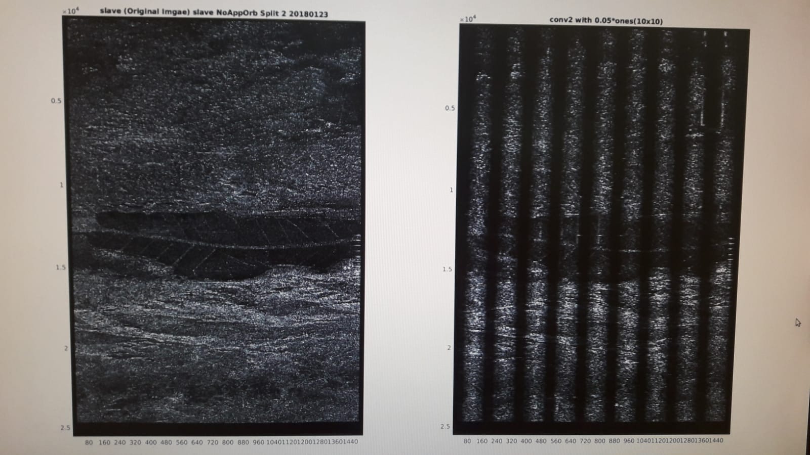
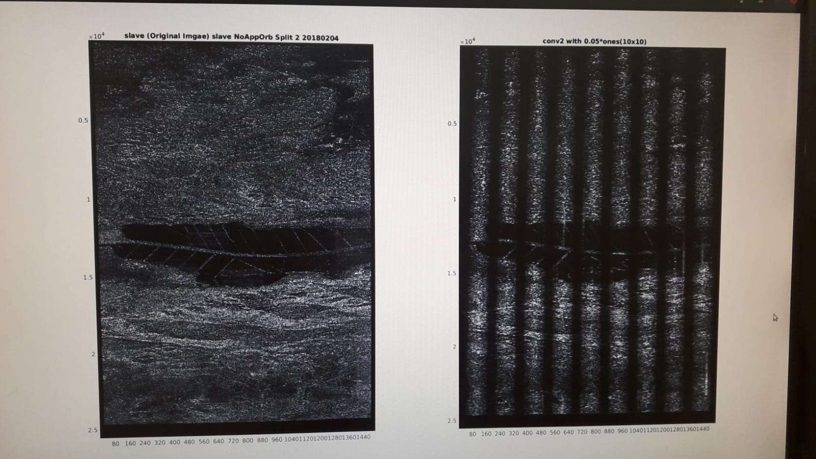
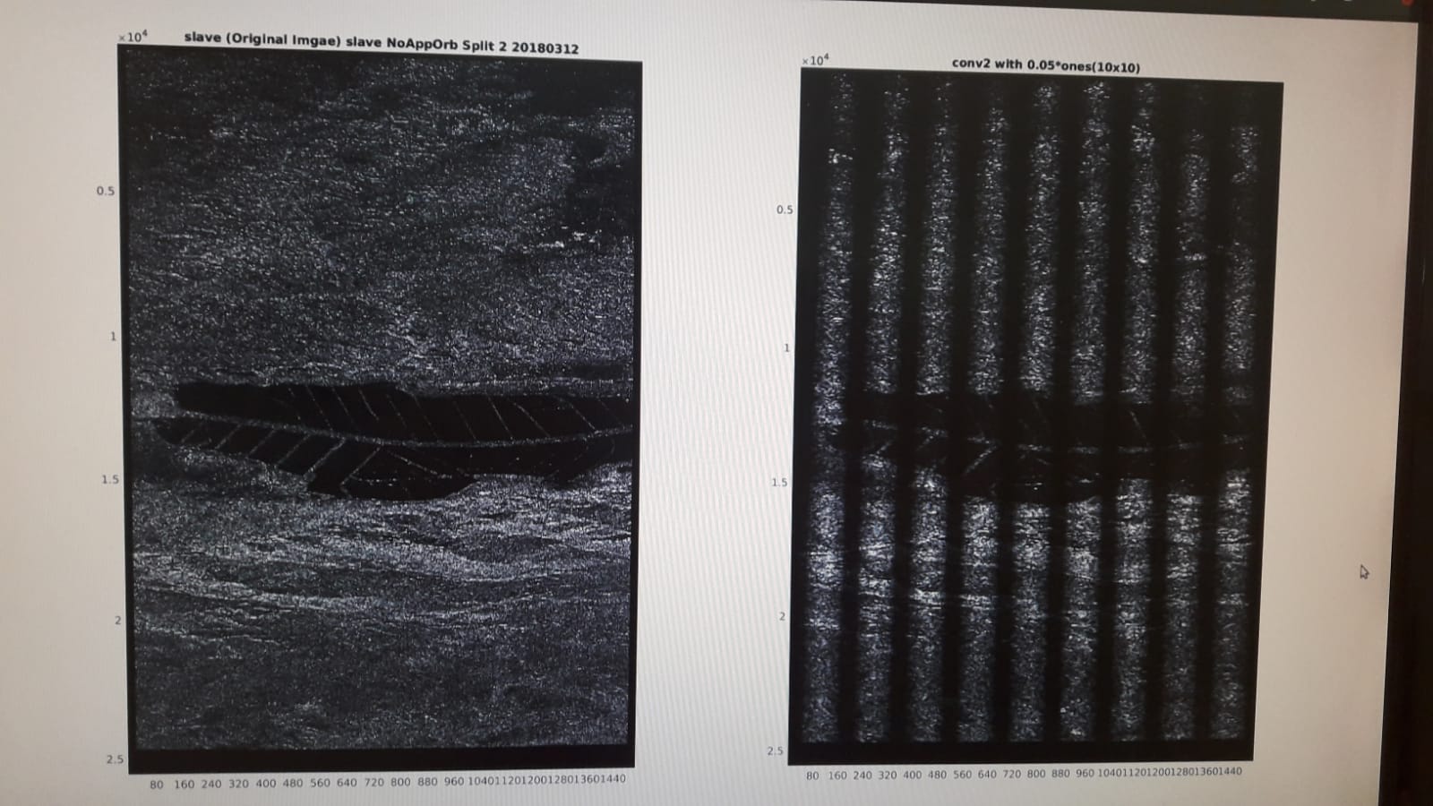
When I looked for the cause, I convoluted the data with a scaled uniform window in order to see the stripes better. I went back stage after stage, and found that every Sentinel raster data (IW SLC) has that stripes, as can be seen in the images below.
The following images were read by SNAP and splitted (due to file size), that’s all.
I then converted it into *.mat files using python library called spectral, loaded into Matlab and made the convolution.
These are images of the southern part of the Dead Sea, taken at 3 different times.
1.
I hope I added some insight to the phenomena, and curious to understand the cause for it.
Oded Horowits
Thank you for sharing these. Is multi-looking or resampling involved in one of the preprocessing steps?
No.
Only loading Sentinel S1A IW SLC data from Alaska Satellite Facility website into SNAP and applying ‘S-1 TOPS Split’ operator, even without ‘Apply Orbit File’ operator
@peter.meadows what do you think this is?
Hi, Can you please indicate which direction is azimuth (i.e. flight time) and range. I’m guessing you are showing just one of the three IW sub-swaths?
Hello @peter.meadows,
Yes, That was IW2 strip #2.
By the way, I checked also IW2 strip #8, to see if the stripes get a different angle. They don’t, it seems very parallel.
Regarding direction, on my images above, the right side was north.
Here is an image from Snap:
The stripes go vertical to the dead sea, so it means that the stripes are parallel to the range axis.
My co-worker hypothesizes that this is related to the curvature of the earth, which is not being treated properly.
Hi, thanks for the extra information - I can see that your are showing just one IW2 burst where range is in the vertical direction and azimuth is in the horizontal direction. So the variation is in the azimuth direction.
I would not expect to see any such variations within a burst (between bursts maybe). I’ve not seen the variations in your image before and so am not sure of what is causing them.
Some suggestions to try:
Hello @peter.meadows,
I was under the impression that the satelite travels in north-south direction (Ascending path and Descending path), and therefore that is the ‘azimuth’ axis.
The whole seen is devided into 3 IW bands (‘IW axis’) , and each band is devided into 9 strips (‘Strips axis’).
Can you please make it clear for me, which axis is the azimuth and which one is the range?
And, what do you mean by ‘the equivalent product processed by ESA’?
Hi,
I was under the impression that the satelite travels in north-south direction (Ascending path and Descending path), and therefore that is the ‘azimuth’ axis.
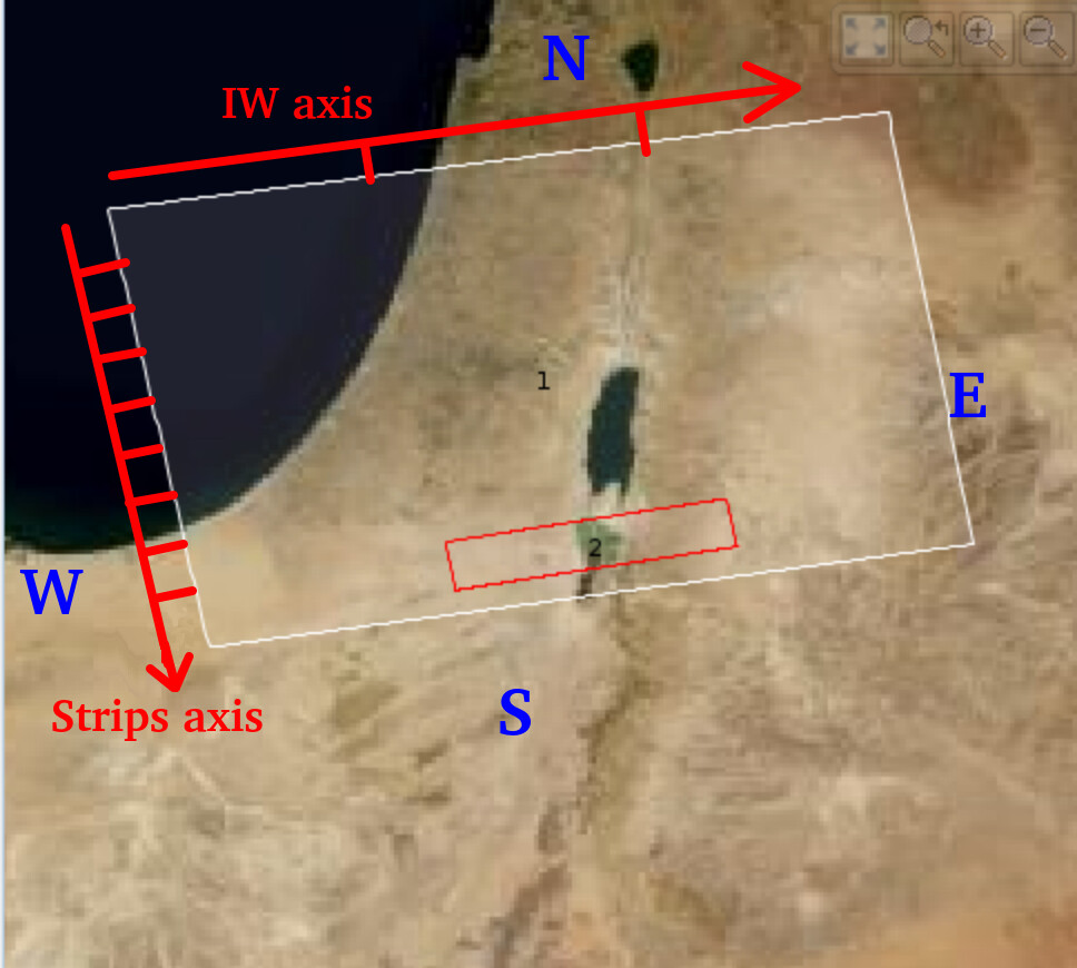
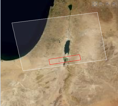
Assuming your white image boundary is correct (I think it is), then the satellite in your image is from an ascending pass (i.e. travelling south to north). Note that the orbital inclination of S1 is about 98 deg and so the ground track moves east to west with time. So azimuth (i.e. increasing flight time) increased from the bottom of the image to the top - see picture below. As S1 is a right-looking SAR, range increases from left to right.
The whole seen is devided into 3 IW bands (‘IW axis’)
Yes - IW1 to IW3 are marked on the diagram.
and each band is devided into 9 strips (‘Strips axis’).
These are the bursts but actually in the other direction you indicated.
And, what do you mean by ‘the equivalent product processed by ESA’?
You mentioned that the product was from the ASF and I assume processed by the ASF. ESA processes S1 data which are available on the S1 Data Hub (The Sentinels Scientific Data Hub). I’m suggesting finding the same ASAF product on the Data Hub (and processed by ESA rather than ASF) and check if you have the same problem.
Could you post the name of the IW product you are using?
Hello
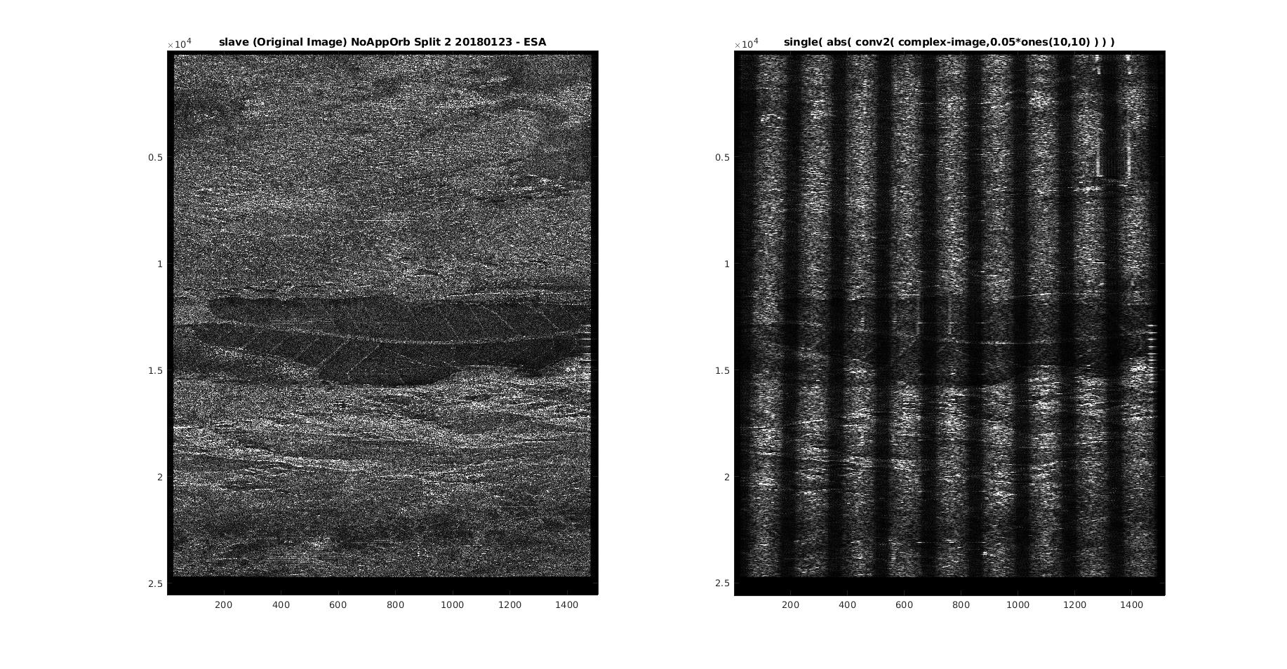
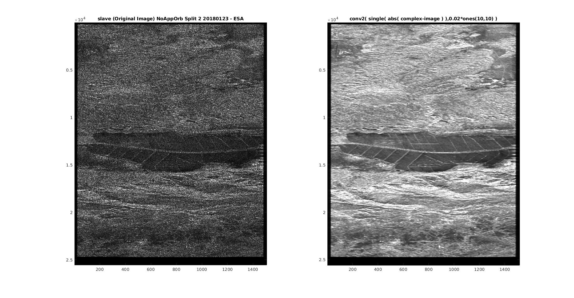
It took a while, but I can say that the results are the same for the ESA product, as you can see in the following image.
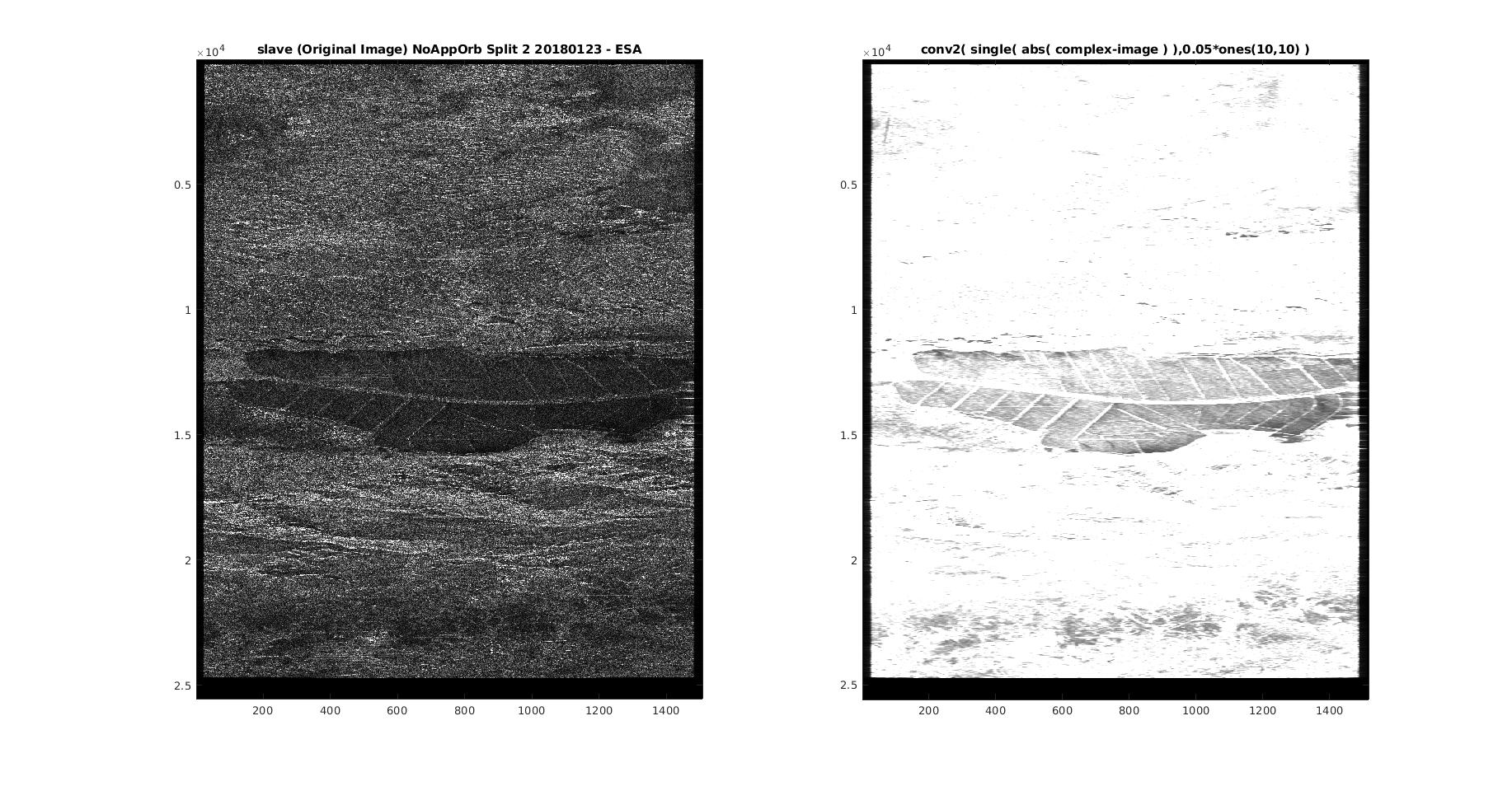
I also want to emphasize that the stripes are seen when the convolution is applied on the complex image. When the convolution is applied on the amplitude only, the striped cannot be seen.
I applied the same convolution windows in both cases, just to make it systematic. If I take a windows with less weigth (0.02 for example), the image is less bright, and no stripes are presented:
Could you post the name of the IW product you are using?
The answer is S1A_IW_SLC__1SDV_20180123T154025_20180123T154052_020284_022A1E_FE4A
So perhaps the issue is related to the convolution itself rather than the data?
I would think that the issue is related to the phase and not to the intensity