Constant offset for GRD calibration

clausmichele · November 4, 2025, 10:54am

Dear all,

I’m working on Sentinel-1 GRD data in EOPF Zarr format and I’m comparing the calibrated products with the one that can be computed with SNAP. I noticed an average difference, where the calibrated values obtained from Zarr are lower on average compared to SNAP.

Looking into the SNAP docs, I noticed this particular sentence: For GRD products, a constant offset is also applied.

However, I couldn’t find any other info on how this offset is computed or where to find it in the metadata.

I probably found where in the code of the Sentinel-1 toolbox this offset is applied but it’s not so clear to me how to reproduce the same in Python.

Can someone clarify me how to compute this constant offset to calibrate the data without using SNAP?

github.com/senbox-org/s1tbx

s1tbx-op-calibration/src/main/java/org/esa/s1tbx/calibration/gpf/calibrators/Sentinel1Calibrator.java

1daae60d5


      
          float[] retroVec1LUT = null;
          if (dataType != null) {
              retroVec0LUT = getVector(dataType, vec0);
              retroVec1LUT = getVector(dataType, vec1);
          }
          final double azTime = calInfo.firstLineTime + (subsetOffsetY + y) * calInfo.lineTimeInterval;
          final double muY = (azTime - vec0.timeMJD) / (vec1.timeMJD - vec0.timeMJD);
          final int[] vec0Pixels = vec0.pixels;
          final Sentinel1Utils.CalibrationVector calVec = calInfo.calibrationVectorList[calVecIdx];
          
          for (int x = x0; x < maxX; ++x) {
              srcIdx = srcIndex.getIndex(x);
          
              dn = srcData1.getElemDoubleAt(srcIdx);
          
              pixelIdx = getPixelIndex(calVec, pixelIdx, subsetOffsetX + x);
              muX = (subsetOffsetX + x - vec0Pixels[pixelIdx]) /
                      (double)(vec0Pixels[pixelIdx + 1] - vec0Pixels[pixelIdx]);
          
              lutVal = (1 - muY) * ((1 - muX) * vec0LUT[pixelIdx] + muX * vec0LUT[pixelIdx + 1]) +
                      muY * ((1 - muX) * vec1LUT[pixelIdx] + muX * vec1LUT[pixelIdx + 1]);

Tagging someone who might know more: @lveci @mengdahl @ABraun @diana_harosa

clausmichele · November 10, 2025, 10:25am

I forgot to post the link to the SNAP docs where this is mentioned:

https://step.esa.int/main/wp-content/help/versions/10.0.0/snap-toolboxes/eu.esa.microwavetbx.sar.op.calibration.ui/operators/CalibrationOp.html

piyushrpt · November 11, 2025, 6:14am

What you probably need is just the betaNought LUT in the calibration XML file. What is the magnitude of difference that you are observing for beta0?

clausmichele · November 11, 2025, 12:20pm

Hi @piyushrpt , I am actually comparing sigma nought values. I leave here a minimal code example to reproduce my current status. What I already checked:

SAFE and EOPF Zarr vales are the same
SAFE and EOPF LUT values are the same

I don’t know how SNAP is interpolating the LUT and therefore there might be a difference depending on that too. Anyway, I still don’t know if there is and how to apply the aforementioned constant offset.

The local geoTIFF has been generated using SNAP 11 and the calibration operator on the original GRD data without any other step, it can be found here: https://drive.google.com/file/d/1KaO26Edzrj4wpE_v2MhStFavFfX1WAhu/view?usp=sharing

import xarray as xr
import numpy as np
import rioxarray
import matplotlib.pyplot as plt

grd_path = "https://objects.eodc.eu/e05ab01a9d56408d82ac32d69a5aae2a:notebook-data/tutorial_data/cpm_v262/S1B_IW_GRDH_1SDV_20170503T173207_20170503T173232_005437_00987B_1A41.zarr"

dt = xr.open_datatree(grd_path, engine="zarr", chunks="auto")

group_VH = [x for x in dt.children if "VH" in x][0]
grd_vh = dt[group_VH].measurements.to_dataset().rename({"grd": "vh"})

sigma_lut = dt[group_VH].quality.calibration.sigma_nought.interp_like(grd_vh,method="nearest")
eopf_sigma_0_vh = ((abs(grd_vh) ** 2) / (sigma_lut**2)).vh.compute()

SNAP_sigma_0_path = "./S1B_IW_GRDH_1SDV_20170503T173207_20170503T173232_005437_00987B_1A41_Cal.tif"
SNAP_sigma_0_vh = rioxarray.open_rasterio(SNAP_sigma_0_path)[0]

SNAP_mean = SNAP_sigma_0_vh.mean().data
SNAP_median = SNAP_sigma_0_vh.median().data

EOPF_mean = eopf_sigma_0_vh.mean().data
EOPF_median = eopf_sigma_0_vh.median().data

print(f"SNAP sigma 0 vh mean: {SNAP_mean} median: {SNAP_median}")
print(f"EOPF sigma 0 vh mean: {EOPF_mean} median: {EOPF_median}")

fig, ax = plt.subplots(1,2,figsize=(16, 8))

eopf_sigma_0_vh.plot.hist(bins=300,xlim=(0,0.2),range=(0,0.2),ylim=(0,10000000),ax=ax[0])
ax[0].set_title("EOPF sigma 0")
SNAP_sigma_0_vh.plot.hist(bins=300,xlim=(0,0.2),range=(0,0.2),ylim=(0,10000000),ax=ax[1])
ax[1].set_title("SNAP sigma 0")

fig.tight_layout()

plt.show()

SNAP sigma 0 vh mean: 0.01803111843764782 median: 0.006793084088712931
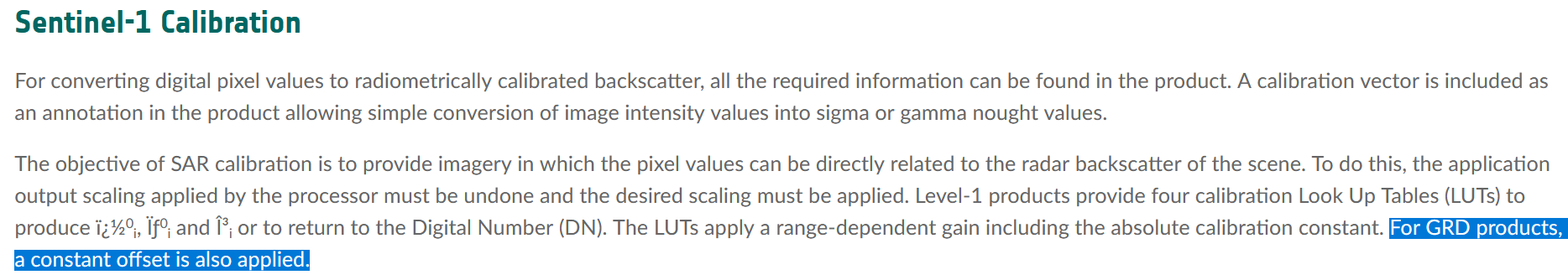
EOPF sigma 0 vh mean: 0.01134358998388052 median: 0.005390457343310118

piyushrpt · November 11, 2025, 4:14pm

You can check that you have wired things up correctly by checking beta0 first. This is a constant value even though it is provided as a LUT. If you see a difference in beta0, the error is pre-calibration or in interpreting the calibration factor. Simple bilinear interpolation is recommended for other LUTs - sigma0 / gamma0 depend on incidence angle which again depends on terrain height used - which is provided also a 1D LUT as a function of along track time.

Best way would be take ratios of the data on the same grid for comparison.

If you read Sec 9.19 of algorithm description document - you will see that the absolute calibration constant K_{abs} is already accounted for in the LUTs.

piyushrpt · November 11, 2025, 9:02pm

You may also want to check your math on abs(grd_vh)**2 . I’m not familiar with how this data is distributed but I suspect that GRD Tiffs are UInt16 and that operation can wraparound if not converted to float first.

clausmichele · November 12, 2025, 10:19am

@piyushrpt thanks for the precious suggestions. You are right, casting to float is necessary:
abs(grd_vh)**2 becomes abs(grd_vh.astype(np.float32))**2. This leads to almost perfect matching of the Beta0 values:

SNAP beta 0 vh mean: 0.028152428567409515 median: 0.01068770419806242
EOPF beta 0 vh mean: 0.028152429574376053 median: 0.010687703824405028

However, Sigma0 values are still off. In the documentation I don’t see the LIA or DEM mentioned for the calibration, but I can find the terrainHeight 1D LUT you mentioned in the metadata. How should I include it in the computation? Can you point me to the right documents?

piyushrpt · November 12, 2025, 3:53pm

You don’t need to use them for computations as the effect has already been included in the LUTs. If your beta0 lines up and sigma0 is off, then the difference is in the LUT interpolator.