I am facing the problem that in my S1 batch processing chain the functions “Remove-GRD-Border-Noise” and “Thermal noise removal” are not working anymore since March 13th 2018.
I receive the error message: [NodeID: Remove-GRD-Border-Noise] java.lang.NullPointerException
Any ideas, if the data has changed or how to deal with that issue?
It is not a problem of RAM since i receive the error on different machines.
Is the problem affecting only images generated since 13 March, or also old images?
According to this link, since 13 March S1 images are processed with IPF 2.90, which has some differences with respect to earlier versions of the processor, for instance in the way noise profiles are annotated in the metadata.
Also, according to this document, starting with IPF 2.90, the pixels in the dark borders have DN=0 (and not DN>0 as in earlier versions, which often caused problems and which SNAP tried to solve with the ‘S-1 Remove GRD Border Noise’ operator).
Maybe SNAP cannot handle property the masking of the border pixels now that they are DN=0?
Just an observation - the S1 Instrument Performance Facility (IPF), the SAR processor, was updated on 13th March to v2.90. The manifest file for S1 products includes the IPF version number. Further details of update can be found at https://www.researchgate.net/project/Sentinel-1-Mission-Performance-Centre.
Hi thanks for the reply,
data up to the 12th of March work fine. So it is quite likely that the change in processing causes that errors. The Boarder Noise is not so critically, since i mask out the data later anyway.
But how to deal with the Thermal noise removal?
Is someone of you from the processing unit or how to inform them about that issue?
Best
Holger
The SNAP team was provided the TN a while ago. Hence, I hope we are close to a solution.
I can confirm that the GRD dirty pixels are also properly cleaned.
Will this new S-1 noise data results in similar noise removal as developed by Nansen Center in
Park et al., “Efficient Thermal Noise Removal for Sentinel-1 TOPSAR Cross-Polarization Channel”, IEEE TRANSACTIONS ON GEOSCIENCE AND REMOTE SENSING, VOL. 56, NO. 3, MARCH 2018 ?
In this paper also azimuthal scalloping noise (due TOPSAR imaging and provessing) is removed.
Cheers, Marko Mäkynen
Any idea on when the update will be released? We’re trying to use S1 GRD in an operational set-up and rely on SNAP to get the latest data processed correctly.
I do have to say that this is quite ridiculous. I do not expect a lot from ESA but at least getting software out in time for the data to be processed should be possible.
Further information on the issues that arose on 13th March can be found at https://qc.sentinel1.eo.esa.int/disclaimer/30/ and https://qc.sentinel1.eo.esa.int/disclaimer/31/. These disclaimers indicate that there could be problems with the noise vectors in the annotation files with IPF v2.90 products up to 2018-03-15 14:01:26 UT (and with auxiliary files S1A_AUX_PP1_V20171017T080000_G20180313T104548.SAFE or S1B_AUX_PP1_V20160422T000000_G20180313T093244.SAFE).
The paper you are referring to is addressing many subjects that are indeed covered by the new IPF version and part of the material is actually taken from the processor algorithm document. For example:
II.A : denoising in range
II.B and III.A - denoising in azimuth. The processor was having natively (i.e. since launch) the possibility to denoise in azimuth but it was an option not activated and the annotations wasn’t providing the azimuth noise vector. With the new IPF this is now the case. The description in the paper looks however correct
The noise power scaling which has been an issue for us (up to the new processor version) and the paper is actually showing well where we were having problems (III.B/C ). The paper is proposing a way to correct for the processor noise scaling issues based on the residual of the demonised signal. The approach can work OK but I believe it is limited to data over ocean. I am not quite sure how it will work over land scenes where we know that even away from noise floor the data is impacted by it .
The new IPF version is the result of a long activity aiming at providing more reliable denoising information everywhere (not only over ocean where it is relatively easy) that I can summarise in 3 steps:
NESZ estimation over the Doldrums, where we have analysed several thousands of bursts to find the few signal-free ones hence giving only noise. This allows to have the best NESZ estimation possible that we use to scale our range profiles. I expect that now the “swath balancing” issue is gone
Find a way to track the evolution of the noise power with the data-take to cope with the earth brightness temperature. In the past we were using only 2 values located at the start/end of the data take. The linear interpolation made between those two point can’t cope with the land/sea or sea-ice transition hapenning.
In order to do that we needed to change the format. The new format introduces the azimuth vectors in the simplest way possible without completely breaking everything. Indeed the format changes are pretty minimum and doesn’t reflect the complexity behind especially for GRD.
The difficulty for GRD relies on the fact that the burst/swath are merged and effective denoising needs to know where the boundary are. Section III.D , overlook the fact that it was almost impossible with the previous annotation to identify burst/swath transition leading to artefacts like fast ripples at swath transitions as you can see them in fig 9. Those should be pretty reduced now.
Furthermore, the swath merging was not constrained and the merging point was constantly varying in azimuth to cope with the roll pointing changes. In the case of EW which has 5 swaths and are 1 min long it was leading to >70 blocks of variable size (some ridiculously small) in where to apply a proper azimuth/range denoising.
We reviewed all that to reduce the complexity on the user side, limiting the number of block to the extreme minimum. Like we did in for range we further add extra point in the azimuth vector at burst transition to avoid any interpolation error. The TN we made available explain how to retrieve them exactly.
The section III.E are also what we recommend to do. We limit ourselves to provide as accurate as possible vectors. Any local correction is let to the user for its own application.
In short, the approaches are complementary. The new products should ease and improve the results obtained in this paper.
Thanks for detailed information!
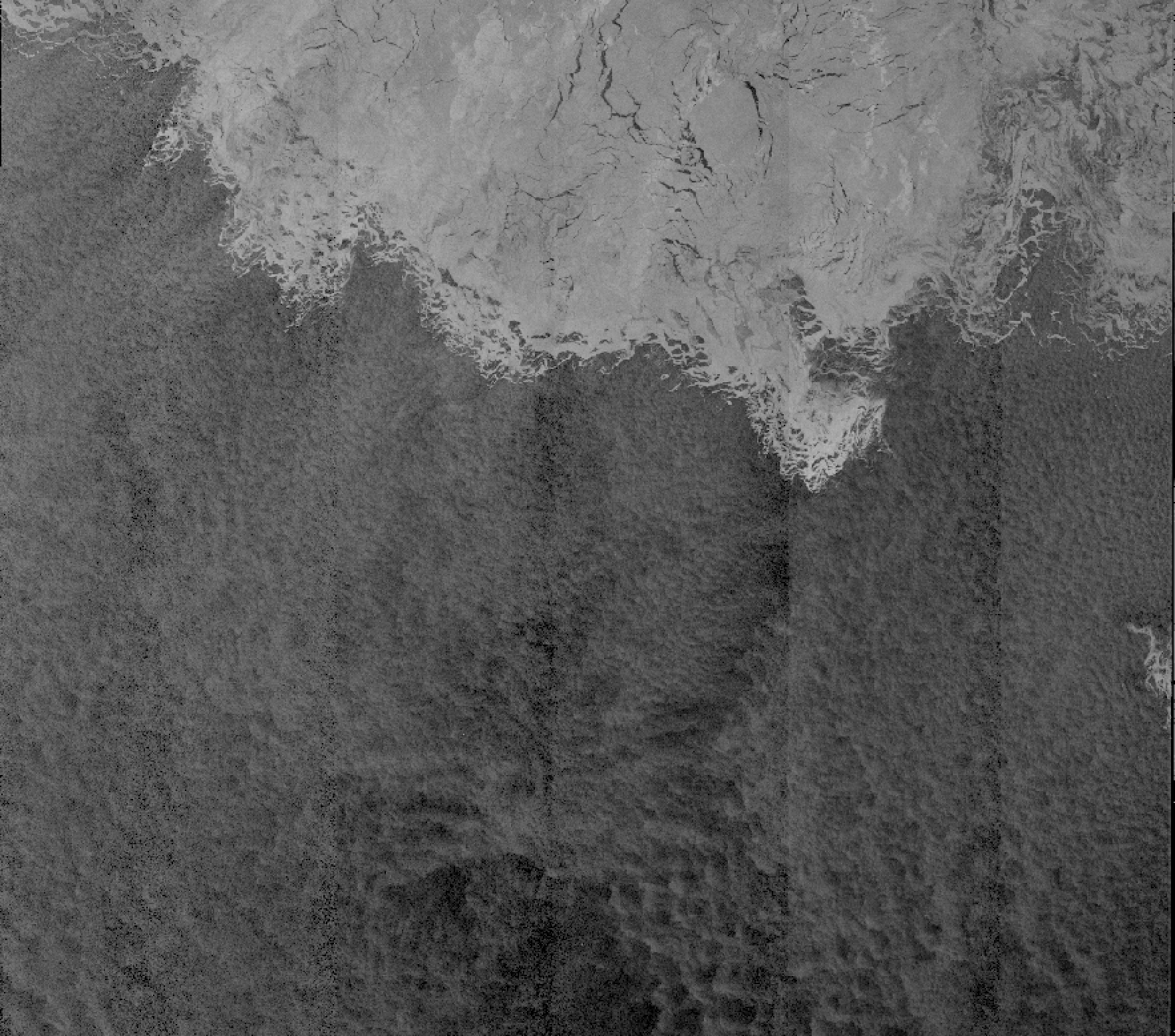
While waiting for the ESA SNAP update, I made a Matlab program to read and process new noise data according to “Thermal Denoising of Products Generated by the S-1 IPF” document. Not sure if I got everything right, but anyway here is a S-1 EW HV image from the Barents Sea having both ocean and sea ice, and the same image noise removed. Calibrated to sigma0 in dB. New noise data improves the image quality a lot, but some defects are still presents, especially boundary between EW1 and EW2 is visible and EW1 has somewhat too high backscatter coefficient level compared to other swaths.
Well done! The approach in the end is not too complex to implement (since we we changed the product to make your life easier).
I have to confess that I am not surprised about your results. We still have to deploy a correction but I don’t believe it will change the overall results. EW is causing some issues that we don’t understand yet.
As you can see in my presentation, in slide 13 there is still a significant residual for EW (not there in IW). This is a point that we need further investigate with the team. However the problem is not so much a scaling issue as reported in the paper but something related to the shape that is leading to obvious residual at swath transition.
For info, could you please give the name of the product you looked at?
The S-1 product was:
S1A_EW_GRDM_1SDH_20180322T044514_20180322T044614_021123_0244CB_E0E2.SAFE
Good news is that scalloping noise seems to be removed with new noise data.
Cheers,
Marko Mäkynen
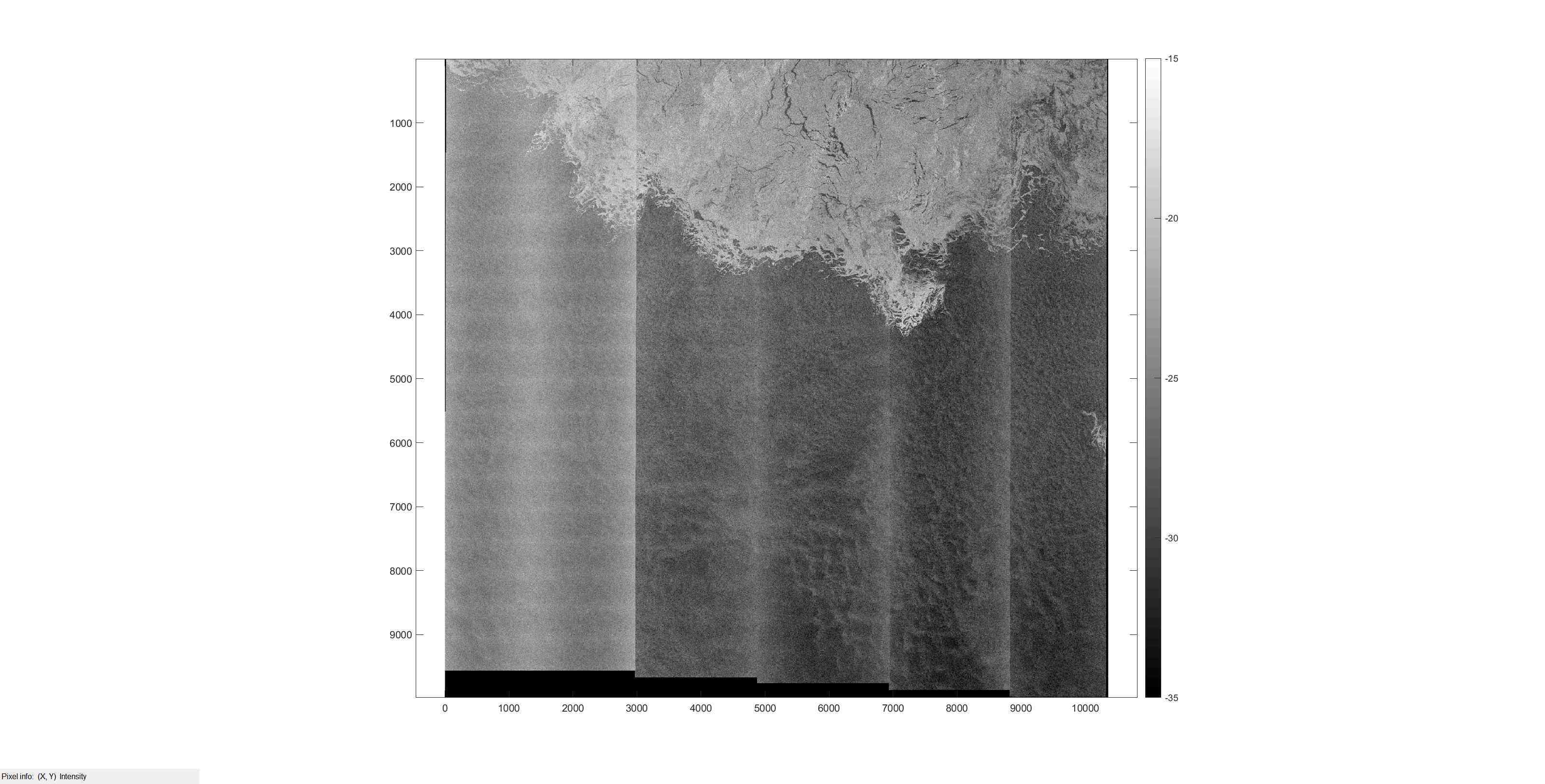
I have used your product as test. The screenshot below shows the denoise cross-pol scaling up the EW1 denoising matrix by a factor of 1.4 (natural values). As you can see, this allows to remove entirely the sub-swath transition for EW1 to EW2.
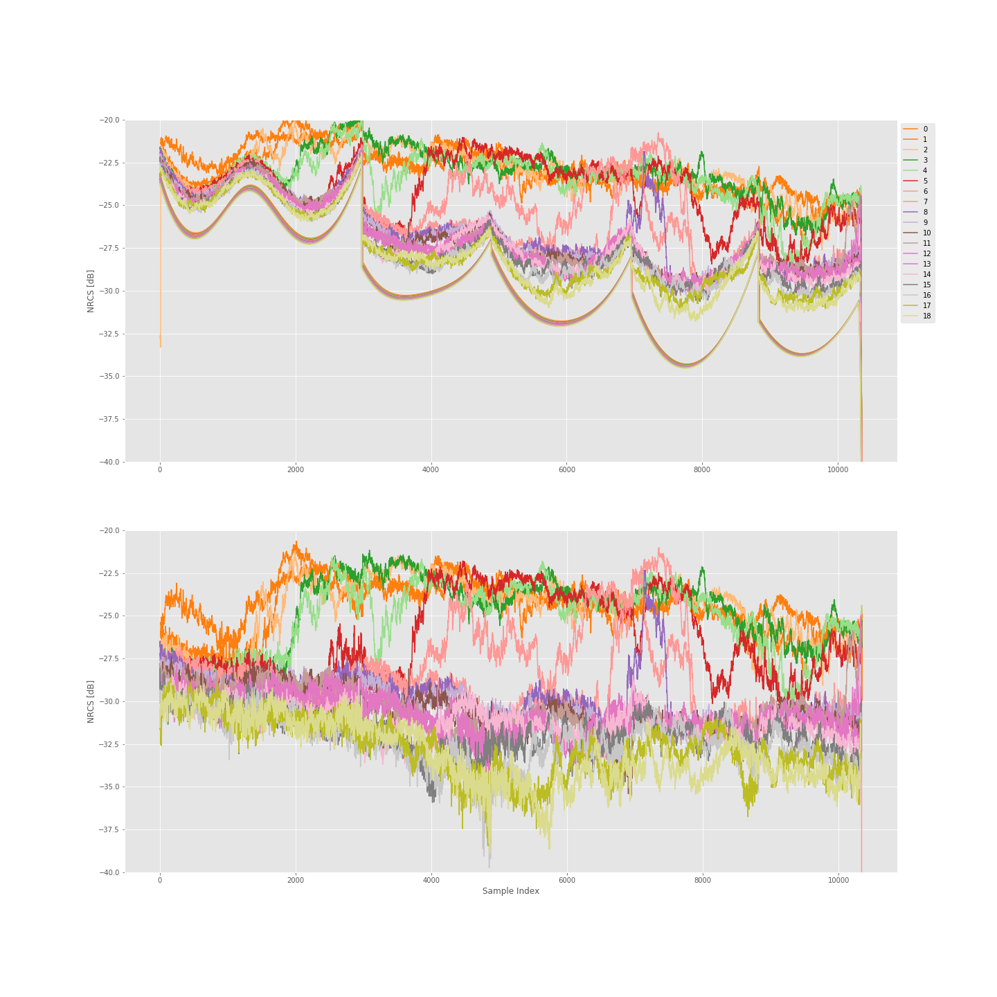
The second plots show the average sigma zero profile in dB before (top) and after (bottom) denoising for different azimuth blocks. In the top plot, the continuous lines represent the denoising profiles for the same block. Scaling EW1 noise by 1.4 means that the we are actually changing the EW1 NESZ values to a level that is 1.5-2dB worst than what we measured over the Pacific ocean (see my presentation slide 13). From the instrument / processing point of view it makes few sense. Hence the questions that we need to understand:
is there any reason why the (especially for EW1) the NESZ figure is different in pacific and up north?
why this difference impacts mainly EW1 and not the others beams (providing that they were all calibrated the same way?
Unfortunately, I have no good explanation for that yet.
The paper you mentioned before is providing a solution to mitigate the effects… locally. By the fact the EW1 NESZ seems to change from a place to another the correction factor provided might not be valid elsewhere. However, pending from an explanation on these issues there is no other solution than scaling the noise vectors locally to achieve smooth NRCS over the swath.