Hi everyone! Well, I have to compare different atmospheric correction methods: Sen2Cor, iCor and C2RCC. My study area is a Estuarine Complex in the Northeast of Brazil, which is caracterized by turbid and productive waters.
With this, I’m turning a 1C level image (Top-of-atmosphere - TOA) into a 2A level corrected image (Bottom-of-atmosphere - BOA).
In order to validate each algorithm, I’m doing match-ups with in situ reflectances. It turns out that the spectral curves look alike (BOA and in situ) - not perfectly but yet almost the same spectral response to a certain band - but magnitudes of reflectance differ a lot from in situ. Here’s one of the lakes I’m using:
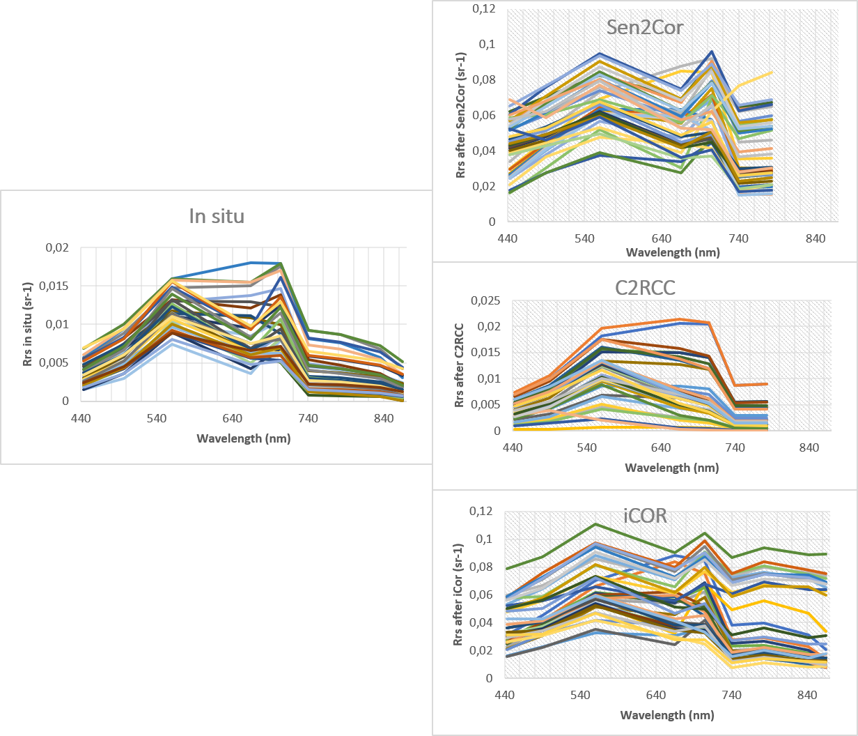
Here, C2RCC seems to have ignored the absorption at 665 nm and Sen2Cor seems to emphasize that absorption. Why?
Some match-ups:
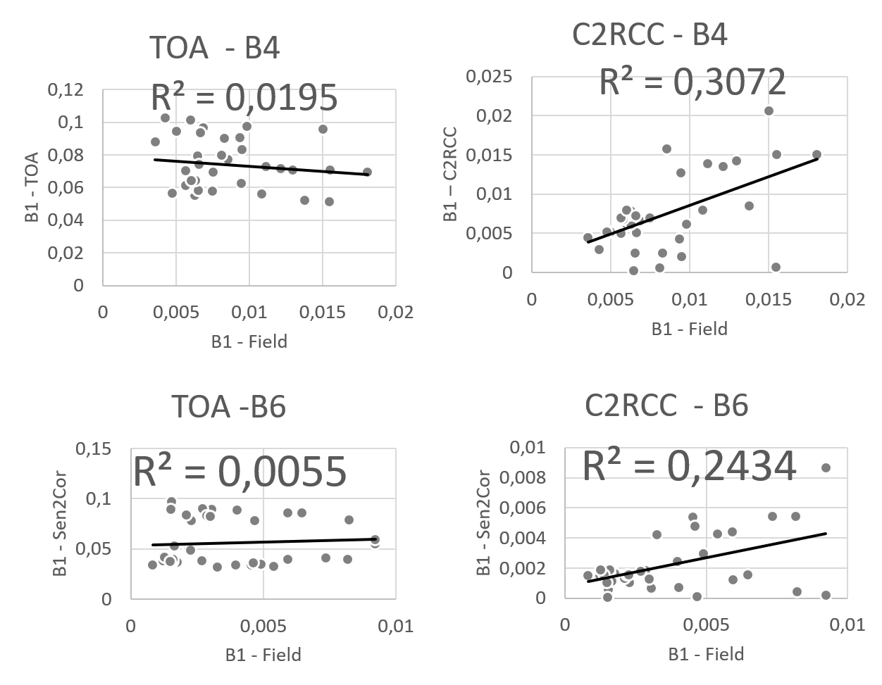
See that C2RCC increased R2 but still there is great dispersion?
So my questions are:
- How can I explain those differences in spectral curves (limnological or atmospheric/orbital explanation)??
- How can I evaluate the performance (in terms of performance metrics) in a way this shape similarity could be represented? (since R2 wasn’t always good)
- How can I explain that in situ reflectances were all under 0,02 sr-1 and the others were under 0,12 sr-1 (except for C2RCC)?