Problem with complex Range Doppler Terrain Correction

Hello,

I am working on TerraSAR-X SAR SLC images, and I encountered a problem during my work. This is not a bug or a crucial issue, but I think it would be worth adding a Warning message about it. For my research, I have to use images terrain-corrected. When using Range Doppler Terrain Corrected in SNAP, one can choose to keep the complex data or not. The intensity value obtained for a pixel is not the same depending on if the complex data are kept or not, and it can be an important difference (more than 3dB). Is this value difference due to that an interpolation is realized on the real and imaginary parts if the complex data are kept and on the intensity if they are not?

I don’t have any opinion if one of the two values is more “physic” than the other, but I think it would be really important to add a Warning message about it to avoid false results. For example, if someone compares two acquisitions obtained at a different date, one terrain corrected with complex data and one without the complex data, the value difference between the two pixels is not only due to the acquisitions.

Here is the example for one images and a selected pixel :

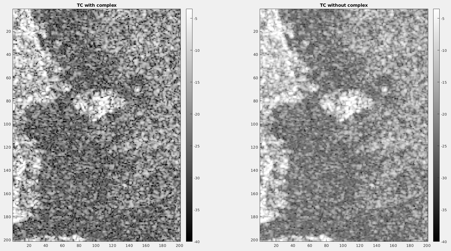
Terrain Correction with complex :

Terrain Correction without complex :

The visual difference for the same area :

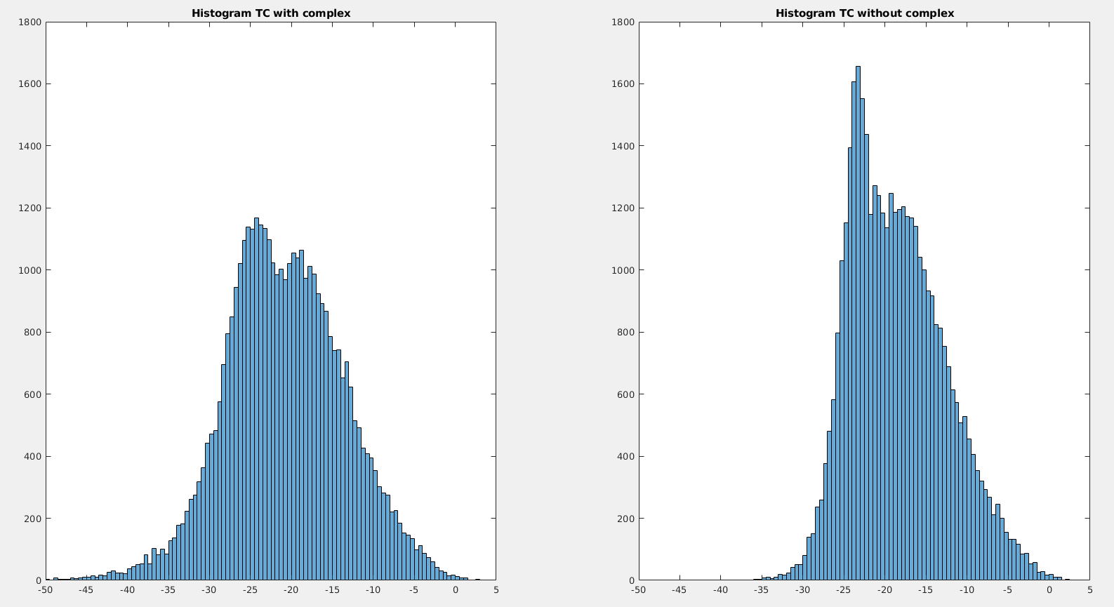
The corresponding histograms :
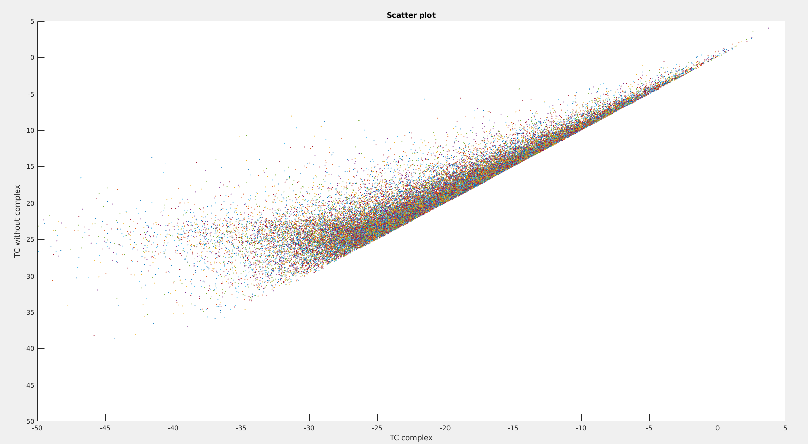
The scatter :

3 Likes

@jun_lu Do you have an explanation?

We will look into the problem. A JIRA ticket ([SITBX-883] TC results are different for intensity and complex output - JIRA) has been created to track the issue. Thank you for reporting the problem

1 Like

One cannot apply standard interpolation operators on SLC since the data is not base-banded. You will need to account for carriers in azimuth and sometimes in range as well, to interpolate SLCs accurately. This is done correctly when generating coregistered SLCs but the generic interpolation approaches used in geocoding modules will not produce good results.

2 Likes

Dear @jun_lu,

I think I have found a clue to solve the problem. As I explained (you can see it using the Matlab code I did to see if I was right), the interpolation between the real and imaginary parts leads to a different intensity than the interpolation of the intensity part. The trend obtained with random values is similar to the one I had with my TerraSAR-X result. I understand that the terrain correction is not a simple interpolation, but I think that the principle is close. The new value obtained for a lat/long pixel is obtained using values from other pixels (selected by the resampling method and the resampling grid), and using the complex or intensity values leads to different results.

I am not a big java user, but if I understood your code correctly (https://github.com/senbox-org/s1tbx/blob/f103f41715ec513db46141f2ada64257bb8d03a5/s1tbx-op-sar-processing/src/main/java/org/esa/s1tbx/sar/gpf/geometric/RangeDopplerGeocodingOp.java), you realize the resampling (line 1570) over I (srcBand[0]) and Q (srcBand[1]) if outputComplex is true (line 603). Otherwise, you only do it on the intensity band (srcBand[0]). Therefore when the intensity is virtually calculated once the terrain correction is over, the result obtained is different from the one obtained resampling the intensity.

Does this information help you to solve this problem? The solution would be to resample over the two source bands (if available) and keep only the intensity if outputComplex is false. But again, I don’t know which one of these two results is the most “physical”.

complexMat=rand(1000,1000)+1i*rand(1000,1000);
intensityMat=abs(complexMat).^2;
[X,Y]=meshgrid(1:1000);
[Xq,Yq]=meshgrid(1:0.25:1000);

realinterpolated=interp2(X,Y,real(complexMat),Xq,Yq,'linear');
imaginterpolated=interp2(X,Y,imag(complexMat),Xq,Yq,'linear');
intensityinterpolated=interp2(X,Y,intensityMat,Xq,Yq,'linear');
intensityinterpolatedcomplex=abs(realinterpolated+1i*imaginterpolated).^2;

figure ; imagesc(10*log10(intensityinterpolated),[-10 0]) ; colorbar ; colormap(gray(256)) ; title('Interpolated')
figure ; histogram(10*log10(intensityinterpolated)) ; title('Interpolated')

figure ; imagesc(10*log10(intensityinterpolatedcomplex),[-10 0]) ; colorbar ; colormap(gray(256)) ; title('Interpolated complex')
figure ; histogram(10*log10(intensityinterpolatedcomplex)) ; title('Interpolated complex')

sz=zeros(3997,3997)+1;
figure ; scatter(10*log10(intensityinterpolatedcomplex),10*log10(intensityinterpolated),sz) ; xlabel('Interpolated complex') ; ylabel('Interpolated') ; title('scatter')
2 Likes

Dear @jun_lu

I think I can confirm my initial hypothesis as you obtain the same intensity values doing a terrain-correction with or without complex if you use Nearest Neighbour (therefore without any averaging on pixel values) as Image Resampling Method instead of Bilinear Interpolation. I hope it helps you with this problem correction.

Hi Paillou,
Thank you very much for your feed back and the analysis of the problem. You are right that the problem was caused by the different handling of the intensity and complex output. We have discussed the issue with ESA scientist. Once we reach a conclusion regarding the right way to handle the complex out, we will fix the code. We’ll keep you and other users update regarding the progress of the issue.

Thanks,
Jun

2 Likes

Based on the feedback of ESA scientists, the following changes have been made to the terrain correction operator:

  1. remove the option for complex output;
  2. if the input product is complex, convert it to intensity internally before applying interpolation.

If you want to use the phase for PolSAR, we suggest you get the covariance matrix first and then apply the terrain correction

Thanks for your feedback regarding this problem.

If I may suggest something, I think it would be good to change the default value for “Image Resampling Method” and to choose Nearest_Neighbour as for most of the other SNAP functions (or to add precision to the Nearest_Neighbour option to specify that it is the “physical” method).
In fact, by doing a bilinear interpolation, we change the pixel values even if the result obtained can be visually better. This modification of the values is very important when one wants to work with the phase.

Thanks for the tip on how to obtain the phase on a terrain-corrected image using the covariance matrix.

@NPaillou Have you managed to terrain correct the covariance matrix? How do you deal with pixel spacing?

Thank you!

@jmbcarreiras I don’t know if it was intended or not (@jun_lu) but it is still possible to output complex data. Therefore I output complex data from my SLC and then create my covariance matrix (manually using Python, but it should be possible to do it using SNAP) from this Terrain Corrected Complex Data.

Could you precise your question concerning the pixel spacing ?

Have a good day,

Nathan

@NPaillou I do get a NullPointerException error when trying to geocode C3 in SNAP.

Don’t you get some sort of internal multilooking when applying TC to your 1-look complex data? I have this ALOS PALSAR scene with 1088 cols and 18432 rows. After applying TC to the 1-look complex data I get 1900 cols and 3477 rows.

Ok I will try to do it myself and keep you informed of the result.
If you select Nearest_Neighbour as interpolation method you don’t do any multilooking.
This is an expected result when doing a TC and letting the initial parameters, what is actually your problem ?

I chose nearest neighbour as the image resampling method and I’m still getting either averaging or sub-sampling.

My problem is that I don’t know what SNAP is doing.

It is subsampling indeed. In few words, SNAP create a grid with pixel size x-y, in ° if you select WGS 84 referential and in m if you select UTM referential for example. This grid cover your whole SLC image. You can select your pixel size, if you don’t enter anything SNAP will select something wider than your SLC pixel size, because it will try to select something which is close to a multiple of your initial azimuth and range size (I don’t know the exact process, you might look at the functions in the SNAP Git).
If you don’t want to have any sub-sampling, you can for example select UTM referential and fix as pixel size the lowest of your SLC pixel size (range or azimuth).

You should try this, and tell me if the output correspond to what you expect.

Ok, that makes sense. I had already thought of doing what you suggest. I’ll give it a try and let you know if the output makes sense.

1 Like

No, the output results in the same size as before, so either averaging or subsampling going on.

Did you use a graph to do it ? If yes, could you show the xml, otherwise could you show a screenshot of the parameters you used please ?

Now it worked, created a terrain-corrected C3 with a pixel spacing equal to az pixel spacing. I’m attaching the graph in case you want to have a look.
ALOS_Cal_C3_TC.xml (4.7 KB)

Ok, so everything is good for you ?

I would just like to add some precisions :
GEOGCS[“WGS84(DD)”, DATUM[“WGS84”, SPHEROID[“WGS84”, 6378137.0, 298.257223563]], PRIMEM[“Greenwich”, 0.0], UNIT[“degree”, 0.017453292519943295], AXIS[“Geodetic longitude”, EAST], AXIS[“Geodetic latitude”, NORTH]]

This line means that you used WGS84 as map projection. Therefore, your pixels are “squared” in degree, not in meters. This means your pixel size in latitude is the one you expect, but the pixel size in longitude is pixelSpacinginDegreePolarEarthRadius PI/180cos(latitude pi/180).
Depending of what you try to do, it might be a problem. If you want pixels “squared” in meters, you should use UTM for example as map projection.

You can find more about this in this topic: