Range Errors between granules in S1-GRD captures

[ferretnt]

Hi,

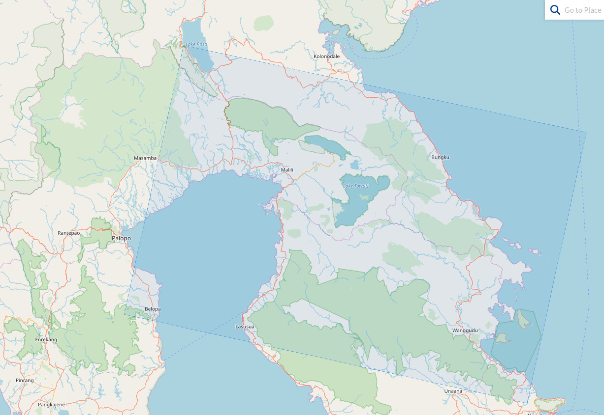
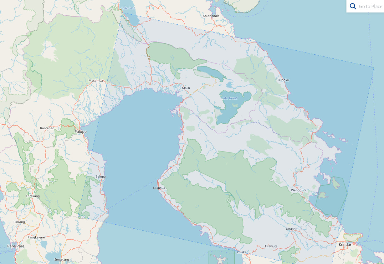
I’m trying to understand what correction (mathematically) still needs to be applied to GRD images in order to project them to a regular WGS84 such that points in a rendered tiff align between different granules. Note that in this case, I’m monitoring the edges of islands, which are (approximately, and certainly to a greater degree than would explain the error I’m seeing) at sea level so there should be no need for DEM-based RTC correction.

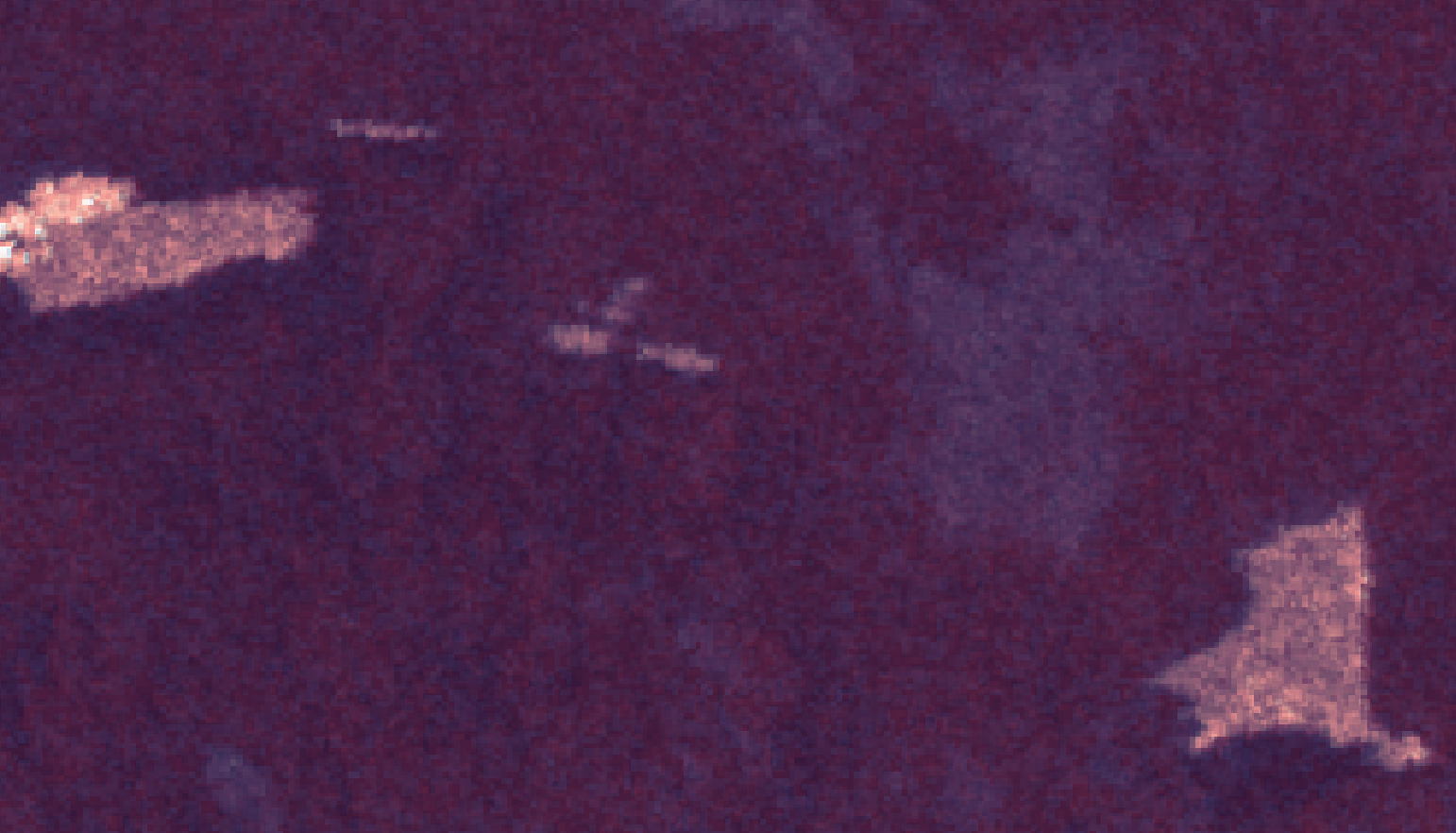
Take, for example, these 2 images, which are small portions on the eastern edge of

S1A_IW_GRDH_1SDV_20250309T213526_20250309T213551_058233_07324A_A474.SAFE
and
S1A_IW_GRDH_1SDV_20250321T213527_20250321T213557_058408_073938_D1AB.SAFE

8_D1AB.SAFE

The documentation about S1-GRD products is extensive, but they’re clearly not quite in WGS84 space. It looks like the azimuth axis is fairly consistent between captures on given track, but the range isn’t. If you then run SNAP’s Ellipsoid Correction->Average Height Range Doppler, everything looks correct afterward, but I’m trying to understand what that’s doing, and why S1 GRD images are in an almost-but-not-quite geographic coordinate system?

I’d like to fully understand how, ideally so I can implement code that handles the final step of projection without having to pick through everything RangeDopplerGeocodingOp.java is doing.

Internally to the vh/vv tiff, what we have is a 2D grid of pixels in range/azimuth space, and then a coarse-ish grid of tie points which map specific pixels to their corresponding X/Y/Z components in WGS84 latlon. Linear interpolation of world-space position is used between tiePoints, which are in about a 20x40 grid. I’m not quite sure why the tiepoints have an elevation but that seems relevant?

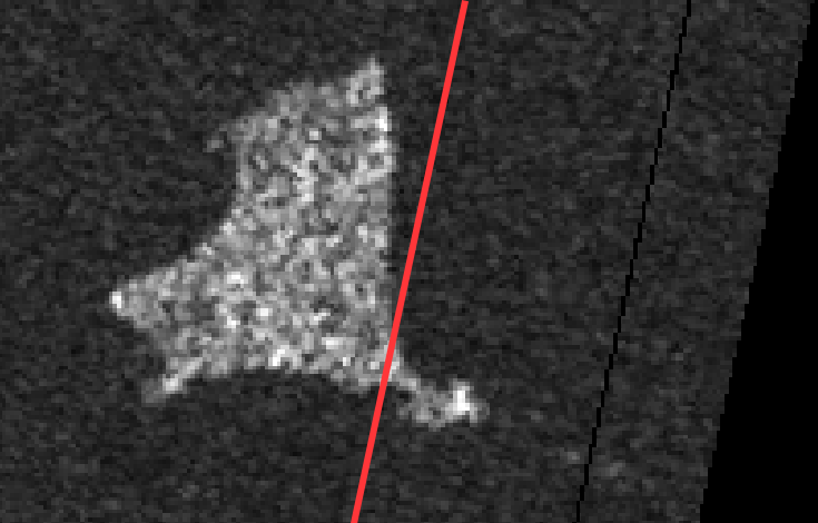
Can somebody explain algorithmically / mathematically what I’m missing? Specifically the errors in georeferencing seem to be entirely in the range direction, and are too large to be interpolation artefacts due to the tiepoint grid being relatively coarse (I also made sure that screenshot was close to a tie point, so it’s not just that!)

To be clear, understanding the math of what’s happening here is more important to me than constructing a processing chain - I know that applying range-doppler correction to all images aligns them correctly, but that’s slow given large numbers of captures, and in my case I expect some (ellipsoid only, not DEM) approximations or optimizations can be made.

Please note that I’m really a 3D graphics programmer by background not a space scientist. Apologies for any incorrect terminology used.

[piyushrpt]

@ferretnt

It looks like the azimuth axis is fairly consistent between captures on given track, but the range isn’t.

There are two issues:

1. Orbits repeat within a tube (say 200 m). Your pixels wont be aligned in range depending on where the exact pass lies within the orbit tube. Azimuth appears to be aligned since the mission is tasked that way to stay in a tube. If you directly align the in image coordinates - range to the targets can be different due to the orbit or choice of near range used for processing.
2. SLC (slant range) to GRD (ground range) conversion involves using a constant height model / slowly varying height model. These numbers used for the processing may not exactly be the same between different passes. They are probably close but not exactly the same. If these numbers are off by a few meters, you should expect a shift of few meters. This difference in constant height model has an impact on relative geolocation. If the GCPs are at different heights, expect shifts.

On the ocean, the DEM is usually assumed to be just the geoid / zero and you can just directly do more stuff with GRD images as the constant height / slowly varying height model works fine in most cases (ignore tides). As soon as you hit land, a meter of height error due to topography will produce a lateral shift in geolocation thats on the order of a meter. This same effect also occurs if different terrain heights were used in SLC to GRD conversion.

This is also why stack generation with SLCs in slant range space is more precise than with GRDs in ground range space - as you will have to undo the constant height model used in SLC to GRD generation if they are different between passes.

[ferretnt]

Thanks very much! I’m still surprised that the edges of those islands seem to be off by on the order of more than a hundred metres, not a few metres - checking the track differences between those captures (assuming I got it right, it did it with a little bit of hacking around with the ASF Vertex GUI) they don’t seem to be that far apart, although I might have got that bit wrong. The full bounding box of the 2 granules listed is sufficiently similar that I can’t imagine an average height across both extents being different.

Is the average ground height used during projection included in the GRD metadata somewhere so that I can check I that was the error? Also, do you know if the actual satellite track is included (e.g. as ECEF coordinates) in the GRD matadata so I can manually calculate the track separation test I half-heartedly did via abusing ASF’s SBAS baseline search.

I’d still prefer to do the reprojection via the existing GRD images rather than doing my own SLC–>GRD projection (the math and code for which is well documented) if possible due to software considerations related to the fact I’m working on an embedded environment for this, and it seems like, given that this is Sentinel-1 data and nothing is really more accurate than about 10m unless you’re talking about interferometry, it should be possible simple to get to a “good enough” projection (again, because everything I’m interested in is at sea level) by applying some lightweight-ish corrections to the relatively small number (<1000) tie points, and allowing them to linearly remap the image during rendering.

[piyushrpt]

The GCPs included in the TIFF files should represent the terrain height model used. More detailed satellite state vectors and terrain height as a function of along track time are included in the annotation xml files.

[ferretnt]

Aha. Yes the tie points do indeed correspond to the terrain elevation used, and they look correct and match if you plot the corresponding positions between the tiffs.

However, the error is clearly a function of the average ground elevation difference between 2 tiffs (based on inspecting a few dozen mismatching and matching cases - note that although my AOIs are all over water, that doesn’t mean the extent of the GRD tiffs the AOI is in doesn’t contain varying amounts of land.) The variation between captures is then in turn is a function of how the track has been cut up with creating VH/VV tiffs. So my assumption is now that each vh/vv tiff is processed using a single average height for range correction. This does seem to match up with the fact that the major errors are noticed when the track is cut differently, such that the iw-vv tiff over an area covers a substantially different area to what it covered in the last granule over the area? In captures that are mostly ocean, this can happen when the number of land (and thus positive elevation pixels) changes because the projected area of the GRD tiff had changed (e.g. the AOI switches from the being at the start of one GRD capture along a track to being at the end of one.)

Do you happen to know where that average height used in GRD correction is stored in (perhaps) the iw-vv.xml files or manifest? IW-VV.xml contains a lot of numbers, none of which look about the order I’m looking for based on averaging the elevations of the corresponding tiepoints in captures.

[piyushrpt]

Terrain height as a function of along track time is provided in the annotation files and along track time is related to line number. These should represent averages over the entire imaged swath in range and an aperture along-track at the given time tag. There should be no discrepancy between vv-vh as these are focused with exactly the same parameters.

Also, you should expect the terrain height to be consistent for the same track / relative orbit. Images from different tracks / relative orbits should almost definitely show larger shifts as the footprint covers a different part of the planet’s surface.

[ferretnt]

Thanks again for all your help. Yes, I see that now. Each geolocationGridPoint in the xml specifies a terrain height, which is identical to the z-value of their corresponding tiepoint in the geotiff. These points match topo, and so their height varies in range as well as azimuth.

What is less clear is the exact meaning of the phrase in the product spec (which is never expanded on): “The ellipsoid projection of the GRD products is corrected using the terrain height specified in the product general annotation. The terrain height used varies in azimuth but is constant in range.”

Two possible interpretations present themselves for how terrain height varies in azimuth. In both cases I’m comparing a number of captures with identical pass and relative orbit:

• The terrain height used varies constantly within a product (?? is interpolated between the values in per line??). A likely interpretation of this is that you should map the (relatively sparse, like 5 per GRD product, so fewer than there are tie point rows) values given in the set of datapoints to produce one terrain height used per row. However, I can’t convince myself that’s what’s happening because I can convert the referenced azimuthTimes from each terrainHeight and confirm that each capture is interpolating a line of near-identical terrain heights at that point in the image, yet the lines that correspond in geolocation produce quite different results if they are at different relative azimuth positions within their products.

• The terrain height for used is a fixed constant for each single GRD product (i.e. one value per vv/vh .tiff). This makes more sense in that it seems to match what I’m seeing. But in that case, it would be nice to know what on earth that average height is. Simply averaging the terrainHeights in the array seems like averaging very sparse values.

To be clear (and I’ll follow up with some images demonstrating this when I have a little more time), I’m not expecting terrain height to be constant between different relative orbits or passes. I believe it is constant for a capture covering identical extent (i.e. same relative orbit and pass, and azimuth start and end correspondonding to about the same latitude.)

I’m surprised, if the height is interpolated within a single image, that same-relative-orbit captures mismatch if they do, and if the height isn’t interpolated (i.e. the interpretation of “varies in azimuth” is “varies once per product”) I’m still struggling to see where that number is documented, or why it wouldn’t be.

[mengdahl]

@nuno.miranda This is getting technical perhaps you can comment? thanks.

[ferretnt]

OK, after further debugging, it looks like the range correction is not constant per GRD product. I now believe it’s interpolated per-line between the relatively sparse terrainHeight values (i.e. my first of the two options above, I previously believed it was the second, but analyzing many more products has convinced me it’s definitely NOT the seconds, and is PROBABLY the first.)

Errors between GRD products with similar swatch “width extent” are typically due to different calculated terrainHeights, and then the interpolation (linear, bicubic, who knows…) between them produces different per-height lines. It is also easy to find examples of products from the same relative orbit where at the north of the image, one image is “east-shifted” relative to the other, and at the south end the shift is westward.

Perhaps, given that this is the SNAP forum, this isn’t even the right place to be asking these low-level questions about the esa-produced GRD products, and I should ask on the ESA earthdata forum. It is surprising that the documentation goes into such great detail in some other aspects, but does not appear to document this at all.

[ferretnt]

Further discussion on CDSE forum confirms that the exact behaviour is not documented. Read s1tbx source for implementation.

Specifics of Range Correction in Sentinel-1 GRD Images

[nuno.miranda]

GRD products are provided in instrument geometry (but ground project).
In this geometry, the only coordinates that really mattera is the SAR timing (range and azimuth times).

I you want geocode the data i.e. warp in geoprojection (UTM or else) you need:

• a flight model i.e. an orbit

• a topography model
  This will warp (range/azimuth) time into lat/lon/height

The orbit provided in the GRD is usually very accurate (cm level) and cannot explain errors of the order of what you observer
However, the height model in the GRD is very coarse e.g. on height per burst. This is not enough for applications looking for accurate position.
The height model is computed interpolating a coarse DEM with the specific spacecraft orbit. Hence it is a different realisation at each processing and I wouldn’t discard differences that could explaining what you see.

You need to geocode the data with a dedicated s/w (e.g. SNAP) and a dedicated DEM for orthorectifying the data.
GDAL (gdal_warp) will read the lat/lon/heigh provided in the tiff tie points and will warp the image it, hence likely using a wrong model leading to the errors you see.

[ghajduch]

I confirm that the height model considered in GRD is very coarse. However, the “coarsiness” of this DEM does not explain the issue experienced here. Even a very coarse DEM should place the sea level close to geoid level, and on the two images pointed by @ferretnt around 40% estimation is over sea. One would expect the location of the GCP provided over ocean to be good enough for points close to sea level. And this is in fact the case here (as confirmed by @ferretnt )

The main difference between the two images is that the two GRD slices are not fully aligned in azimuth due to variations of acquisition plan during the two acquisitions.

First image

Second image (significantly longer)

The issue is here mostly related to the way GDAL is by default warping the image using the tie points provided in the product. It performs an interpolation of the lat/lon position of each pixel of the image.

The culprit is here the way this interpolation is performed by GDAL *by default*, not even forcing that the interpolation is matching the lat/lon vs row/line provided in the list tie points (!!). Then slightly different slicing of GRD products will lead to different way of performing this interpolation and hence different results of wraping.

Considering the “Thin Plate Spline” option of GDAL Wrap you will get much better results.

See below a color composite of the two images (one colored in blue, the other in red with transparency) once wraped with Thin Plate Spline option, illustrating a proper geographic matching for the two GRD products.

Those two products with a different spatial coverage just allow to pinpoint that GDAL wrap needs to be used with caution and with the proper options. Once done, depending on your application, the flatness of your area of interest and your target geometric accuracy, a complete orthorectification is not necessarily required.