Sentinel-3 SLSTR Level-2 LST problem with clouds and temperature amplitude

[Dreamlone]

Hello, dear colleagues!
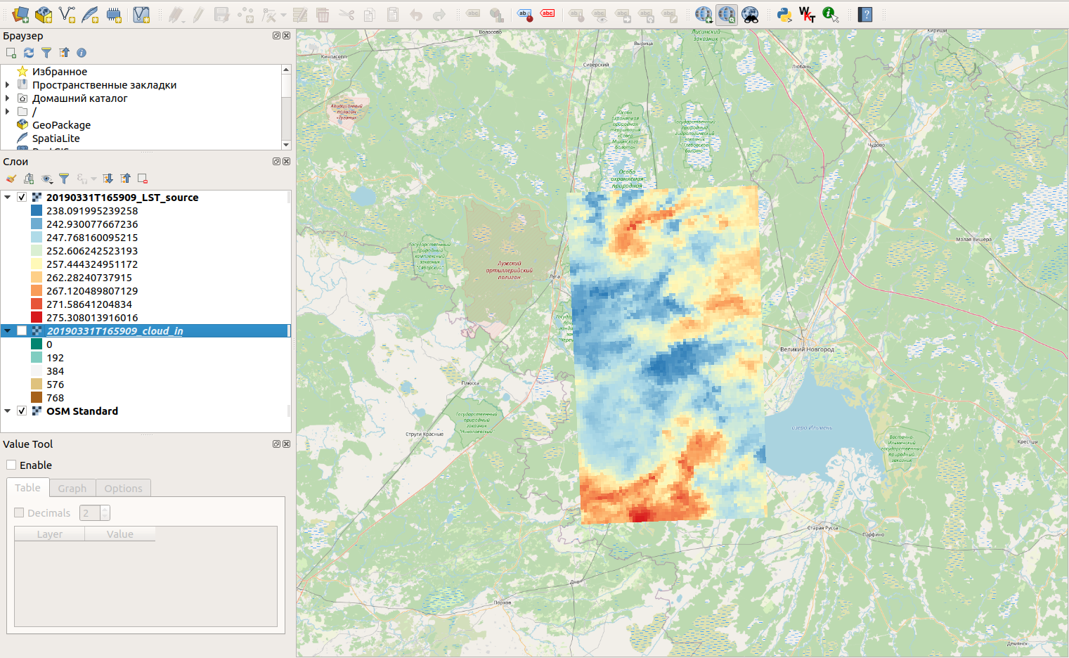
I work with data from the Sentinel-3 satellite system, namely Earth surface temperature (LST). This is SLSTR level-2 data.
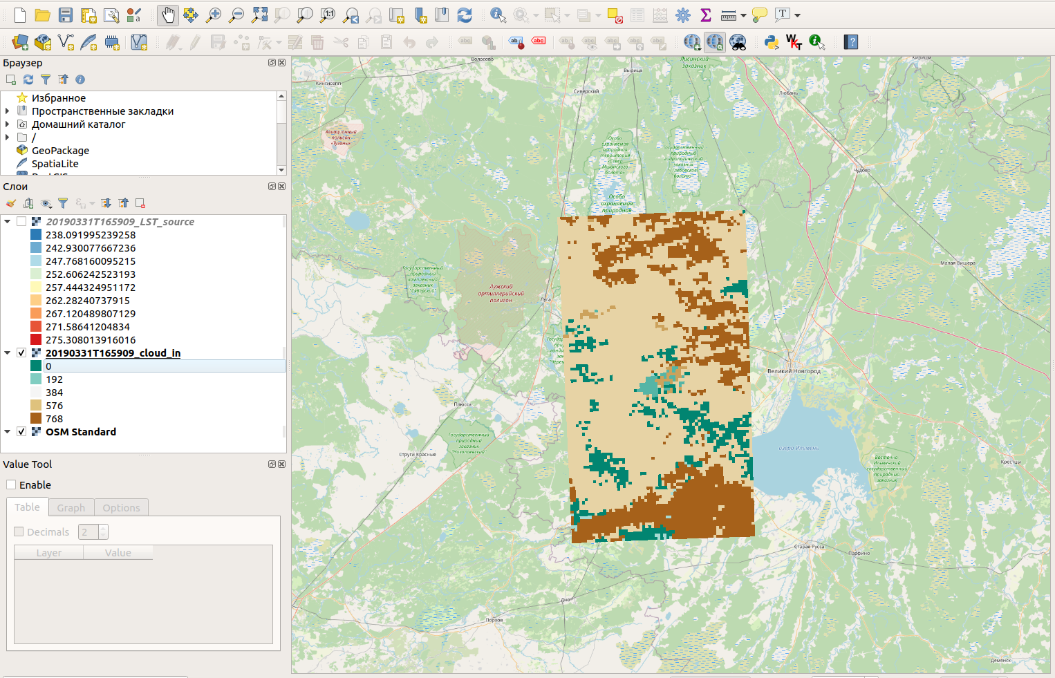
I have a problem - I can’t determine where the clouds were in the picture. In the source archive, I found a large number of additional matrices that can be used. The layer most similar to a mask of clouds seemed to me - “flags_in” - “cloud_in”.

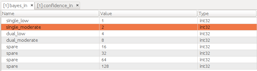
But the problem is that I could not find any information about what codes mean what. The decryption that is presented in the preview function on the web service https://scihub.copernicus.eu does not correspond to reality: there are codes in the layer for which there is no description. For example, for cloud_in there are notations: 1 2 4 8 16 32 64 128 256 512 1024 2048 4096 8192 16384 32768, but I have codes 0, 768 …

I decided that perhaps all values that differ from 0 in the cloud_in matrix are clouds, and with this cloud mask I cut off all those pixels on the LST matrix that have a code other than 0. But when I checked, I found that with the received there is something wrong with the layers of temperature. For example, I have an image for a territory located a little south of St. Petersburg (Russia) on March 31, 2019. And almost all the temperature in the image is much lower than 0, in some pixels - -33 degrees Celsius.

The temperature in the picture is measured in degrees Kelvin.

This certainly could not be. Even in all the images, the temperature amplitude is very very large, sometimes it can change by 30 degrees in one pixel in a day. Moreover, the temperature of water bodies (surface water bodies) is in many cases negative.

I checked the Sentinel images with the MODIS images, and it turned out that MODIS did not catch anything like that, everything was quite good - the water temperature was above 0, etc.

Please help me deal with this issue. Maybe I’m somehow not marking the clouds in the images. What layer (and what values in it) do I need to use for the cloud mask?
Or is it because of satellite, and such strange results are a feature of the sensor?

P.S. I work with files using Python

[dtlloyd]

Hi,

If I understand correctly, you wish to “decode” the “cloud_in” band of Sentinel 3 to identify the location of cloudy pixels in your image, preferably using Python.

As a brief aside, level 2 WST products have a “quality_level” mask with a simpler classification: the band pixels are values 0 - 5, with 5 being the highest quality indicator for the sea surface temperature.

For level 2 LST products the situation may be different. In processing Sentinel 3 level 1 products I found a way to extract a reliable cloud mask from “cloud_in”. However, I have yet to find a good resource explaining the process for decoding “cloud_in”. For the solution I derived in Python I use a function adapted from Landsat 8:

def _capture_bits(arr, b1, b2):
    width_int = int((b1 - b2 + 1) * "1", 2)
    return ((arr >> b2) & width_int).astype('uint8')

Through investigating with various values of the parameters “b1” and “b2” I have found:

cloud_mask = _capture_bits(cloud_in_array,1,0)

yields a simple, useful cloud mask for Sentinel 3, where “cloud_in_array” is the array extracted from the “cloud_in” band. Each pixel then takes one of four values: 0,1,2,3. I find that any pixel with value greater than 0 reliably corresponds to clouds. It’s likely that the “cloud_mask” array this produces is the similar, but not the same, as what can be derived from the BQA band of Landsat 8 (with different values for b1 and b2), where the equivalent “cloud_mask” for Landsat 8 reflects a probability of clouds for each pixel.

That all said and done, there is almost certainly a way of decoding “cloud_in” that the original developers intended that likely differs from the above. I would happily stand corrected if someone else has a better approach and can share it here.

[Dreamlone]

Hello, thank you for your answer!

The information you gave me will be very useful. Unfortunately, I am now faced with the task of automatically applying a cloud mask using only ‘SL_2_LST___’ data without using additional remote sensing products.

At the moment, my code looks like this: https://github.com/Dreamlone/SSGP-toolbox/blob/master/SSGPToolbox/Preparators/Sentinel3/S3_L2_LST.py
I use the code LST_matrix[clouds > 0] = CLOUD VALUE to determine where the clouds are in the image and where they are not. But I’m not sure if I understand the encoded values correctly.

Moreover, in the data ‘SL_2_LST___’ in flags_in.nc - there are layers where there should be information about the probability of attributing a pixel to the cloud. I tried to figure out the values in the ‘probability_cloud_dual_in’ and ‘probability_cloud_single_in’ matrices, but I didn’t succeed.

I will definitely write a few words on the forum about how I solved the problem (if I can solve it :)).

[Dreamlone]

Hello, dear colleagues!
Update: I addressed this question to Copernicus EO Support, and received an answer.

"To mask the clouds in the LST you should either use one of the two masks:

• bayes_in_single_moderate

• confidence_in_summary_cloud

These are separate approaches to cloud masking. The single_moderate mask is a probability based mask designed for LST, whereas the summary_cloud is a combination of all the threshold based land masks in the cloud_in variable.

When you selected which mask to use then clouds are detected if the mask is set to 1."

Since I use Python to automate the data processing, I use the following approach. I download the archive, then open a NetCDF file in which I access the “flags_in.nc” array, in it I refer to the matrix “bayes_in”, then I use the value 2 as the cloud presence identifier. So, the path is flags_in.nc - bayes_in - value 2
And then: LST_matrix[bayes_in == 2] = GAP, so I got a cloud mask.

I hope my post will help someone deal with cloud flags in LST data

[ABraun]

Thank you for your sharing this answer.

[Dreamlone]

Another update

Dear colleagues, after working with the Sentinel-3 LST data, I decided to add some information.

1. It is better to use both cloud masks at the same time, because if you use them separately, some incorrect pixels may remain in the image. I’m not sure that this approach will work for you, but I did it for my research.

2. A little bit about processing. As it turned out, in the matrices that can be used to determine cloud cover, the information is encoded as follows.

Codes in matrices are represented as 1, 2, 4, 8, 16… so that the sum of these terms is unique. In other words, if the matrix contains the value 3, it means that the pixel is encoded with the values 1 and 2; 7 can be decomposed as the sum of 1, 2 and 4, and so on.

So, if you open the sentinel-3 LST layers via SNAP, you can see the description of the codes.

For the bayes_in matrix, the cloud code (single_moderate) is 2;

For the confidence_in matrix, it is 16384. You need to look at these matrices and look for which cells can contain these codes. For example, if we take the bayes_in matrix, where the cloud code is 2, then we need to consider all cells that have values as clouds 2 (2), 3 (2+1), 6 (4+2), 7 (4+2+1), 10 (8+2) etc.

You can do this in python using numpy arrays.
For example:

bits_map = np.array([‘O’, ‘O’, ‘A’])
clouds_bayes_in = bits_map[bayes_in & 2]

Now you have a matrix where the clouds are marked with the value “A”.