Background
Surface velocity remains a key parameter of the ice-sheet dynamics as they represents the direct response of the ice-shelves’ health. The easiest way to obtain bidimensional velocity is by using feature-tracking-like techniques. SNAP has such a function.
The pixel-offset module developed in snap is defined by a number of parameters :
- Grid Spacing (in azimuth/range) : The grid azimuthal/range spacing in pixels (1 pixel = 10x10 meters in GRDH images).
- Registration Window Size : The window width and height for cross-correlation.
- Cross-Correlation Threshold: Threshold for normalized cross-correlation (NCC) value. If the cross-correlation value is greater than the threshold, then the estimated offset is considered valid, otherwise invalid, resulting in a gap in our grid.
- Average Box Size: Size of sliding window for averaging offsets computed for valid offsets.
- Radius for Hole Filling: It defines the size of the window for hole filling. For invalid offset, a window with given radius centered at the grid coordinates is defined. Offsets from valid neighbours within the window are used in interpolating the offset for the current grid coordinates.
We’ve also managed to modify the source codes of SNAP. This enabled us to export the azimuth shift and range shift raster images. In addition, we re-enable a hidden functionality to let the user select the oversampling factor used.
In short, the algorithm will look for each grip location the shift of range and azimuth that maximizes local correlation. This shift is considered as a bidimensional displacement. In order to get a better estimate of the 2D-shift, the search window analyzed is oversampled. The default oversampled value is 16 in each image direction. Said in other words, using default oversampling parameter, the smallest shift is a sixteenth of a pixel. Using GRDH images, it means a 0.625 meter shift in azimuth or range direction. Using a revisit time of 12 days, it means that the smallest detectable velocity is about 19 meters per year. More precisely, detected displacement are integer multiples of 19 meters / year. When resampling the grid to the input image resolution, pixels will be interpolated between this discrete set of values. However, areas of low displacements (between zero and ten meters per year) greatly suffers from this limitation. The algorithm is not able to detect the rich fineness of the ice-flux, crucial for locating precisely the ice divides. These ice divides are the regulators of the total mass flux of huge ice basin. Their location is important for the initialization of ice models.
In our modified version of SNAP, the user is able to set the oversampling factor to 2, 4, 8, 16 (default) , 32, and 64.
It is important to note that if setting a oversampling factor to 64 allows to detect displacement of less than 5 meters per year, it is also much more computer expensive.
In this short analysis, we would like to see the influence of the oversampling factor on overall results. We also want to see if increasing the oversampling factor above the default value brings valuable information. In other words, are the potential improvements worth the time invested ?
A second question to be answered is the choice of the post-filtering parameters, aka hole-filling and spatial averaging.
Oversampling Influence
The first element to consider is the computation time. This element is crucial because it helps decide either or not we will put large efforts to produce potentially finer results.
As we can see, at low oversampling factor, among the processes involved in the offset tracking module, the cross correlation step is negligible. However, at oversampling greater than 16, the cross correlation step becomes the major component of the algorithm.
From figure 1, we can observe that oversampling highly increases the fineness of the displacement detection (red rectangle represents default value). Figure 2 shows that above-default value brings subtle changes in low velocity areas.
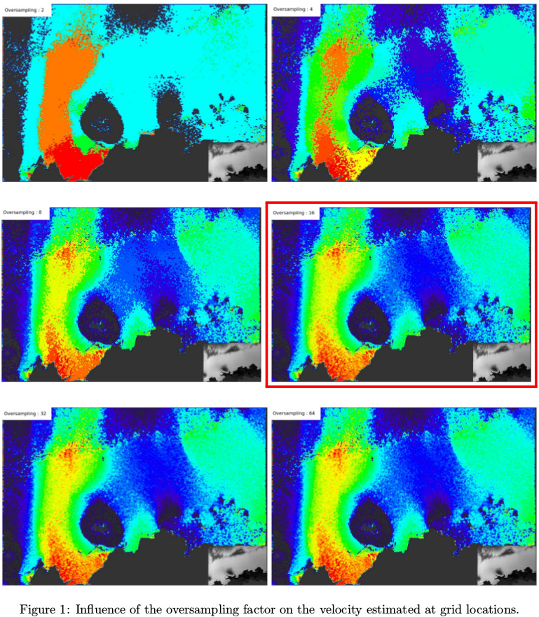
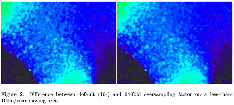
Figure 3 shows the way the oversampling factor discretises the range of detectable displacements. Our study area is moving at a maximum of about 300 meters per year, mostly in azimuth direction. Using 12 days pairs, we can expect a maximum displacement of about 10 meters, i.e. the image resolution of Sentinel-1 GRDH acquisitions. That explains why, with an oversampling factor of 2, only velocity of 0, 150 and 300 meters per year are found. With an oversampling factor of 4, we also allow the detection of 75 and 225 velocity meters per year displacements.
Increasing the oversampling factor allows to detect more subtle changes. The default value (16) allows the measurements of about 19 meters per year velocity (figure 3, red rectangle). Increasing again adds fineness in the results.

Post-Filtering
In the end of the algorithm, SNAP has a grid whose values are an estimation of the 2D displacement. This grid is not perfect for two main reasons :
- When the correlation between master and slave patches is too low, the shift found is considered as unreliable and dismissed. It results in a hole in the grid. Using inverse weighted distance around the hole, the algorithm tries to compute the missing offset. The default value is 4, meaning that the offset will be estimated with shifts up to 4 grid locations away.
- Detected displacements using cross correlation of SAR images produced very noisy patterns and false positive detections. Average filtering consists in a low pass filtering the grid according to a certain convolution window size. The default value is 5.
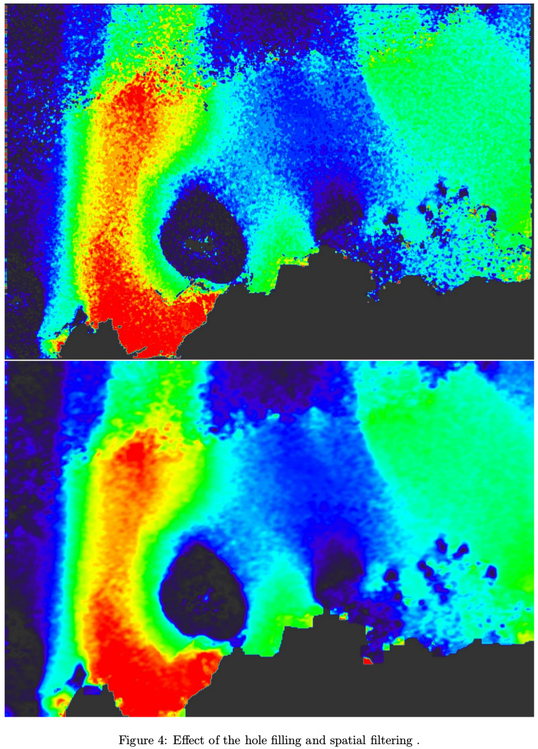
As we can observe in figure 4, the SNAP post-processing (especially the spatial averaging) greatly reduces the displacement noise but also increases a lot the “blur effect”. The hole filling has almost no influence of the results.
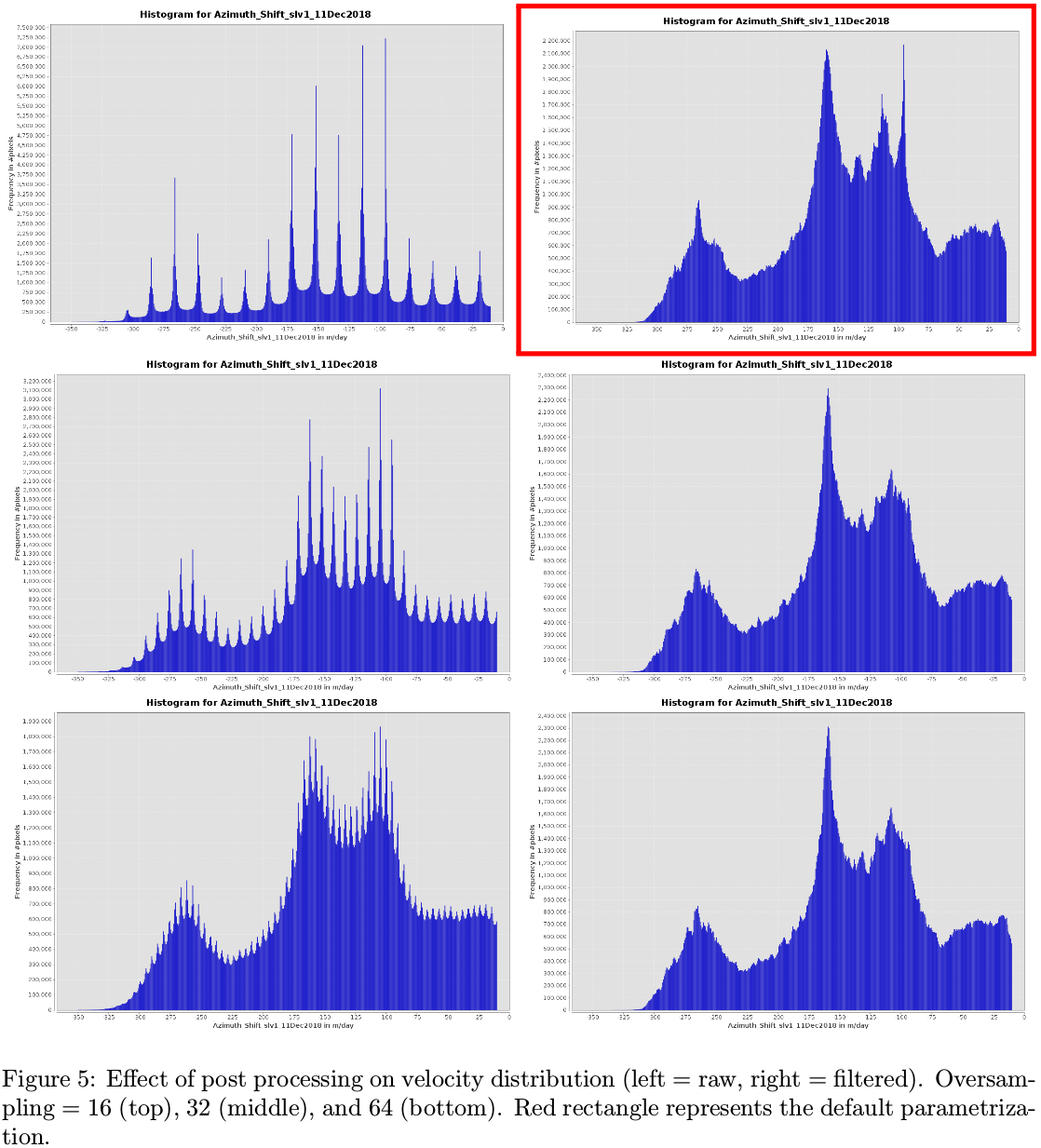
Looking at the velocity distribution, post filtering is also a way to enlarge the range of possible values (see figure 5, from left to right). However, the filtered distribution is dependent of the raw distribution. While the filtered distribution of results from an oversampling 32 or 64 are similar, the 16-fold oversampling creates a strange peak.
Remarks and Feedbacks
As we can observe, the oversampling parameter is an important element in the offset tracking algorithm. The balance between fineness and computation time is part of the equation but we would have appreciated to be able, as a user, to set this value to fit our needs. For the displacement detection of the jakobshavn glacier, it is sure that the default oversampling factor is more than enough. However, in most of the part of the Antarctic Ice-Sheet, this is too coarse.
Concerning the post-processing, as a researcher, it is sometimes better to have access to the raw results and do whatever is needed to make the velocity usable in our very specific context.
Fortunately, SNAP saves as CSV file the entire set of velocity estimates. It means that it exists a way to obtain these raw data. Nevertheless, there are formats much more suitable in geosciences to store a set of formatted and auto-documented 2D arrays : the netcdf. Netcdf would greatly helps the transfer of data from the remote sensing community to modellers.
Finally, it would be great if SNAP would be able to apply the Offset Tracking algorithm to debursted SLC images in order to take advantage of the very good range resolution of Sentinel-1.
EDIT : I totally forgot to thanks the developers who, by their hard-work, managed to help hundreds of users to get their hands on SAR data.
 If I can be useful in anyway, I’d be happy to offer my help