The top one is the ascending and descending time series deformation for a single point.
The bottom one if the accumulated deformation for the piece of highway Rome-Fiumicino derived from the vertical deformation velocity during all the time series.
I have not saved any scripts, as both plots were specifically done for that study. Probably I will regret not had saved those scripts.
oh thankyou. if you can ,i want to know what should i do in the stamp to produce a time series picture.i use the function “ts”,but i can’t get the graph like the first one.
I have some questions regarding the ps_plots that can be obtained in Step 7 of StaMPS. I just want to know the exact meaning/interpretation and significance/role of the following ps_plots to better arrive with reasonable results: ‘u-d’, ‘u-m’, ‘u-o’, ‘u-dm’, ‘u-do’, and ‘u-dmo’. Among these, it says that ps_plot(‘u-m’) can be compared with ps_plot(‘u’). Moreover, if ps_plot(‘u-m’) looks generally smoother then ps_plot(‘u’), then unwrapping was done correctly.
Also, I did analyze one site before using SARPROZ. I know that SARPROZ and StaMPS have different PSI algorithms/implementations (and may give different results). I reanalyzed the same site with StaMPS (same SAR scenes and master scene). Both captured the subsidence bowl. However, I just noticed that for SARPROZ (even with SqueeSAR), the displacement history always starts at 0 from the first SAR scene. For StaMPS it is not the case. I am curious about this difference.
This is related to the reference value which can be set by StaMPS individually. If no point is selected, StaMPS takes the average value of all PS instead. It is discussed and explained here: How can I define reference area in SNAP - #6 by falahfakhri
So when you select a suitable point, your time series will start at 0.
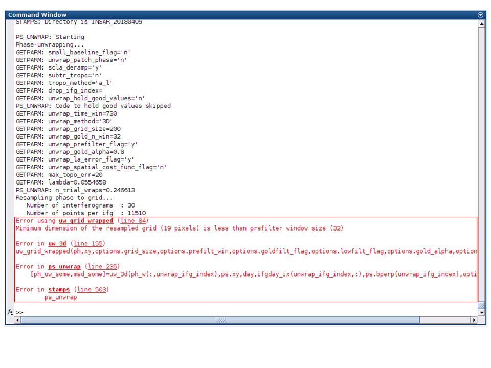
You’ve also answered the same issue. Unfortunately, after setting the value from 32 to 16 to 4, the error still occurs. What other way I can fix this error? It happens in STEP 6.
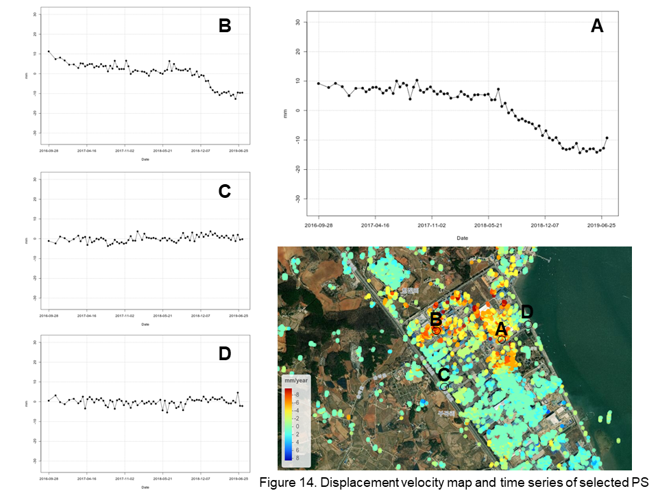
I selected a suitable point as my reference point for my study area and set the following:
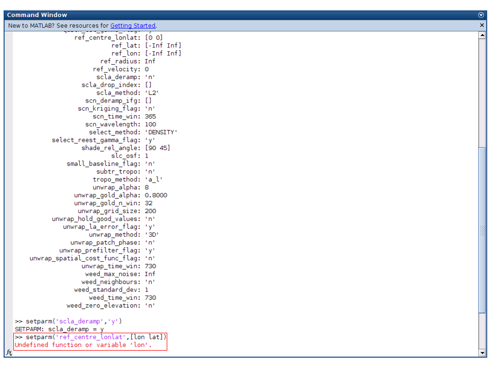
setparm(‘ref_centre_lonlat’, [lon lat]) Note: I’ve set the values for [lon lat]
setparm(‘ref_radius’, 40)
While doing so, I did change also some of the default values for some parameters (i.e., scla_deramp, unwrap_gold_n_win, unwrap_grid_size, unwrap_time_win, scn_time_win).
Somewhere around A is the location of my selected reference point as this region shows insignificant deformation based on SARPROZ and SqueeSAR results. As you can see, the displacement time series for point B did not start at 0 value in the first SAR date. I was expecting it would after following your suggestion. I wonder if I did follow it correctly.
Or maybe I can just subtract the value of the first SAR date from the rest of the points to get the red dashed line.
Hi @ryeramirez, first, nice to see that you use StaMPS-Visualizer for your work :). I encountered the same issues as you describe here and I always subtracted the offset from the first date from the wohle time series to get the plot you want to see.
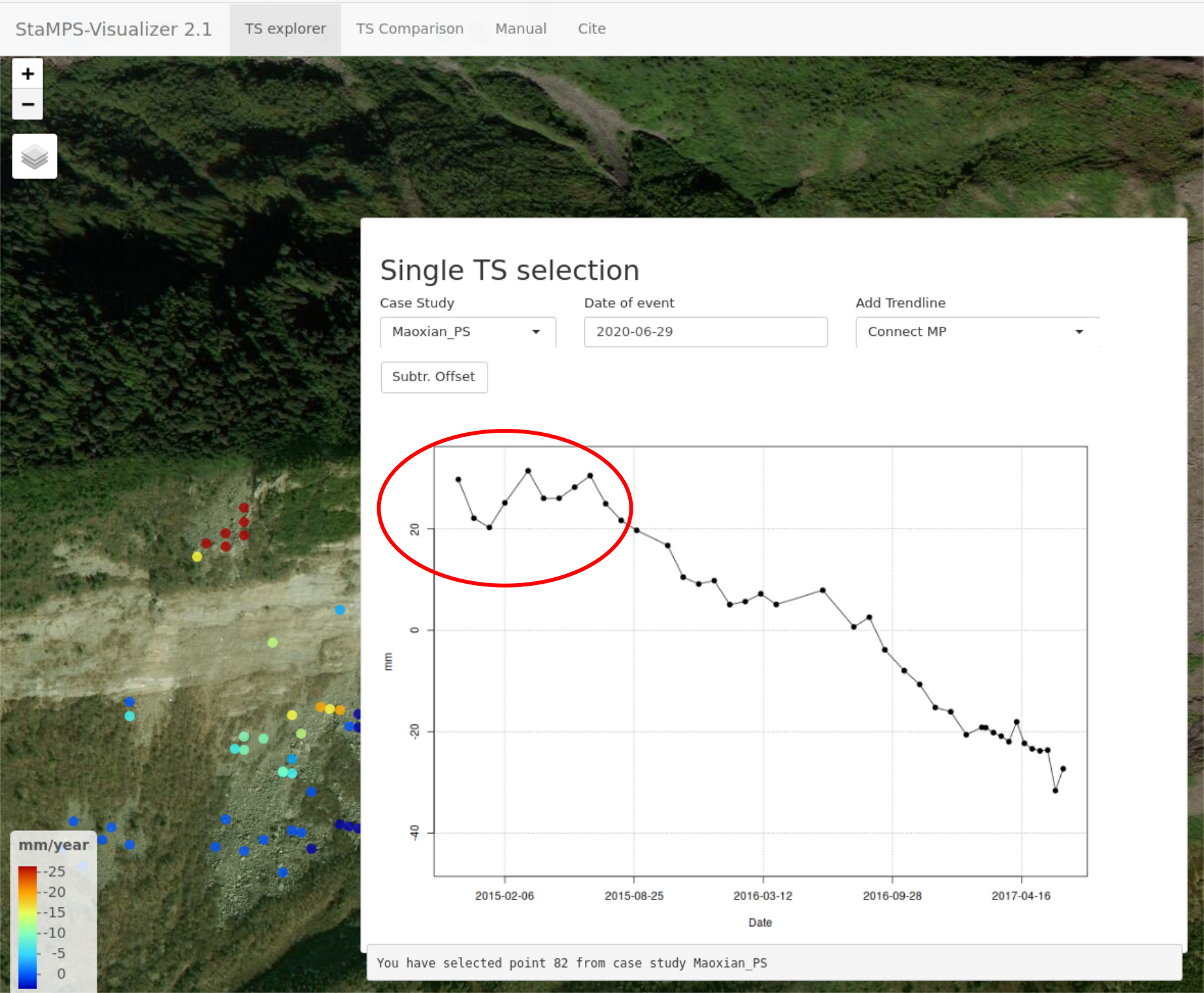
StaMPS-Visualizer uses the export from StaMPS as they are, without handling the offset, and as I understand StaMPS, it alwas uses the master date as the reference and probably that is where your time series crosses 0 in your plot. Since we want to show a trend , related to the first date of the series, it makes much more sense, to finally present the data with respect to date 0 and not to master date.
One more thing that I find a bit nicer to look at, is to use 2nd order polynomial trend line (also provided in StaMPS-Visualizer) instead of the date-to-date connection. outliers like in the end of your series would be still present as data points but the trend line would describe the real movement more realistic. Just a thing which came to my mind when looking at your results, which are very nice by the way
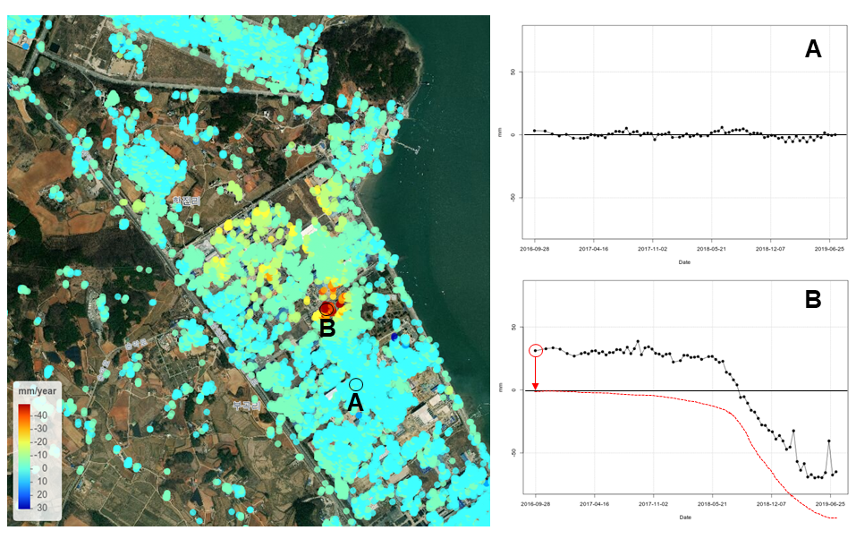
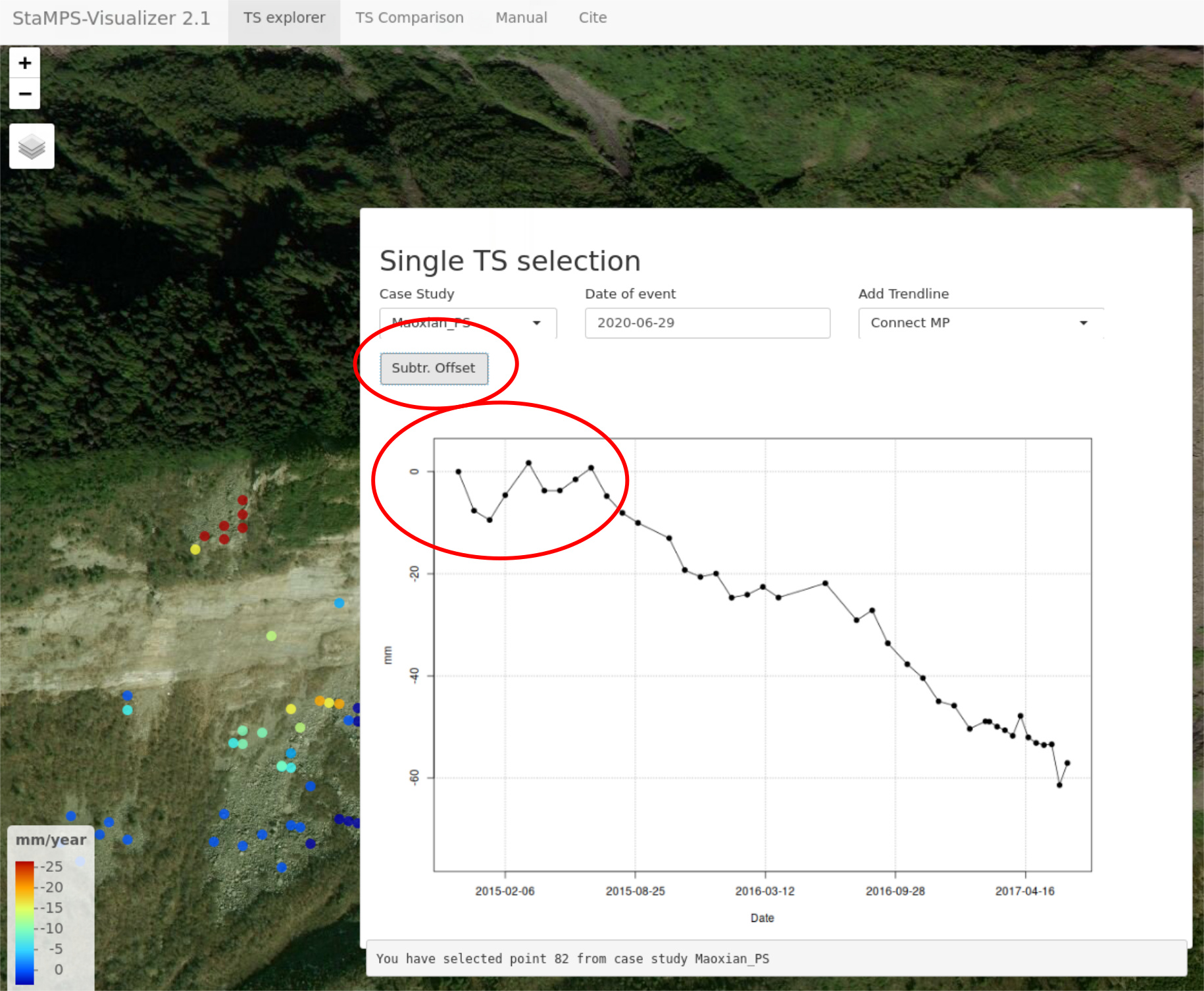
Your problem motivated me to add a new feature to the StaMPS-Visualizer You can now use the “Subtr. Offset” Button to subtract the offset like you described it to align the time sereis to be 0 at the first date. Example:
The old way, before you use the Offset button (still available and the default plot after you select a point):
First, thank you for providing us this great visualization tool for StaMPS-derived results. It’s really very nice. I think I have to upgrade from the beta version to the latest one (v2.1).
Also, I am just curious if StaMPS also provides the temporal coherence of the selected PS? Or is it assumed that we do get relatively high temporal coherence with just using the ADI?
I have one suggestion also (since I am not a programming expert). Would it be nice if StaMPS-Visualizer can generate a smooth pixel-based displacement map overlaid with a displacement contour?
That I do not know, I have not seen an objcet like that, but it is worth to have a look into the objects within the Matlab environment after you have run StaMPS.
Actually, I once started programming a 2D KDE to interpolate the points, hopefully I will find the time and add this feature, contour lines from those interpolated raster should be no problem, thechnically, but I do not know if this is helpful every time. However, there are many potential improvements for the visualizer.
Thank you for giving some light on this. Because in SARPROZ or even in SqueeSAR results they provide temporal coherence of the PS points.
Anyway, I have one concern regarding the CSV file. I know that the first two export_res_XX correspond to the lon lat coordinates of the points. I just wonder if export_res_3 corresponds to the displacement for the first date? In the StaMPS Visualizer, there are 77 date-to-date points but in the CSV file, after the first two export_res_(1 and 2), I have 78 data points.