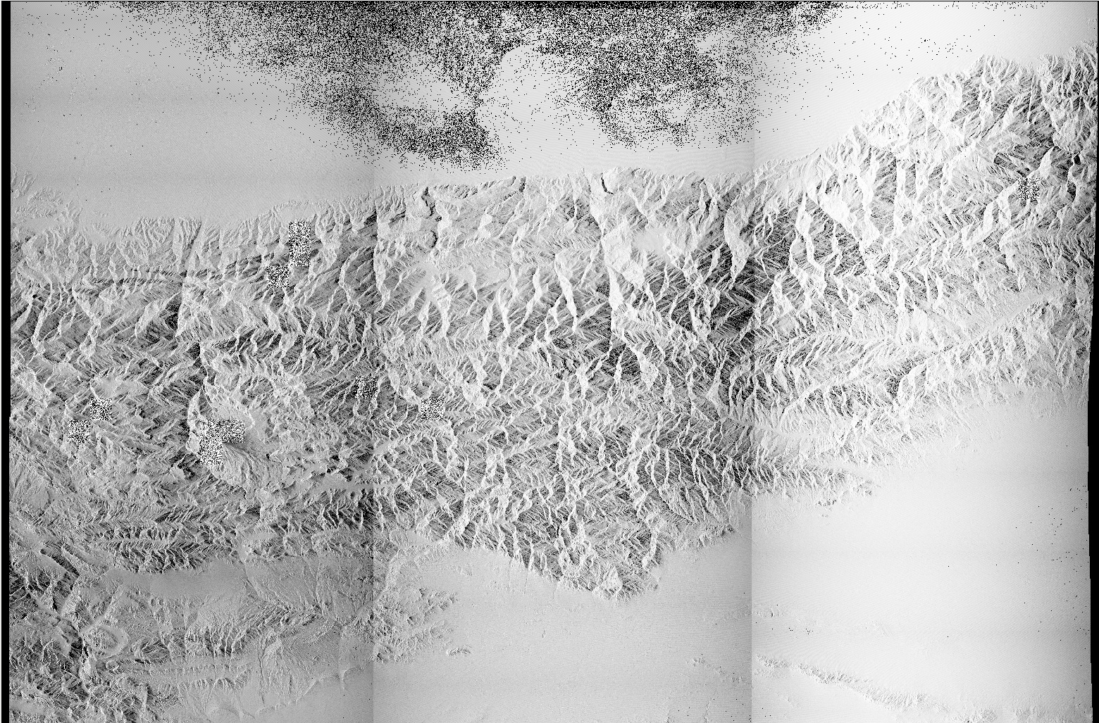
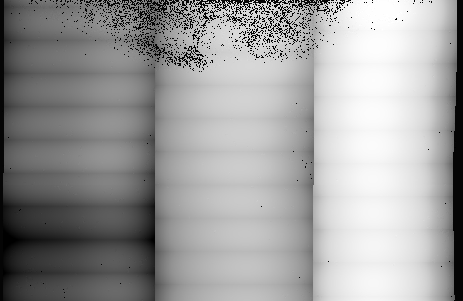
The image below is the difference of the images from the two graphs above, and what I expected from the difference from the top two graphs. (zeros shown black in Caspian Sea area)
The topography in the residual in the first image is normal. It was introduced by the Terrain Flattening operation in which the beta0 is normalized by the local illuminated area simulated using DEM. The output of the first graph can be mathematically expressed as (DN^2 - noise)*cal/sim where DN^2 is the intensity of the image, noise is the thermal noise, cal is the calibration factor and sim is the simulated local illuminated area. The output of the second graph is (DN^2)cal/sim. Here we can see that the residual is given by noisecal/sim where sim is simulated using DEM and mimic the topography. That’s why we see topography in the residual.
Thank you Jun Lu. Mathematically that makes perfect sense for the current implementation in S1TBX.
Empirically, I believe there should not be any component of thermal noise that is relative to sim: noise*cal/sim. Sim should only be related to topography and observation parameters. Possibly, terrain-flattening should be applied before thermal-noise-removal. That is a question for a more senior radar scientist than I.