I am studying the variation of radar cross sections on a specific place. It helps me and my collegues to validate model predictions. My study area is extremely flat (20 meter height difference over 300 km long).
From my knoledge in the domain, using sigma0 takes into account the acquisition geometry, since the reference surface is the ground. With that in mind, I expect that using different orbits or mixing ascending/descending should not influence much the sigma0 in case of “no surface change”. Please correct me if I’m wrong. i’m more into interferometry and things like that are more recent to me.
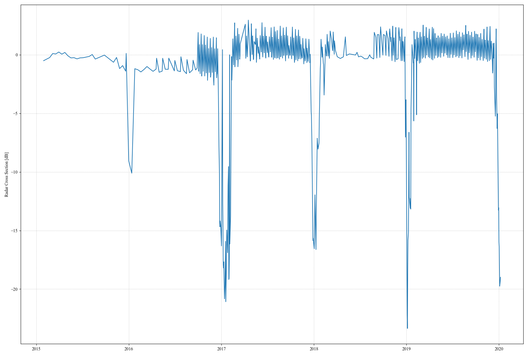
My study area is a bit boring, in the sence that nothing really happens except in case of strong melt events that can be identified by peaks on the graph. In the beginning of the time series, only one satellite on one single orbit was usable. Without considering melt-events, things are quite calm. Then, mid-2016, a second orbit is added over my study areas, and we can already see the up-and-down pattern. With the addition in 2017 of S1B and new orbits, it became crazy.
If I restrain the time-period in 2019 (without melt-events), we can clearly see that there is a ~2dB serrated pattern, that do not correspond to a S1A - S1B potential bias. Example for the May 2019 time period, we have more S1B than S1A.
With sigma0 the radiometry is corrected for the ellipsoid only. If you want to “correct for observatio n geometry” you need to use gamma0 aka. radiometrically terrain flattened data. When this is done properly you may mix obervation geometries for intensity data with rather good results.
Hi, All land surfaces show a variation in sigma0 with incident angle (i.e. position across the swath). This is likely to be the cause of the variation in sigma0 you show in your plots since you have a mixture of relative orbits in your list of dates.
I suggest you plot sigma0 for each relative orbit seperately (you can find the relative orbit in the product manifest file - also all products from the same relative orbit will have been aquired 6 or multiple of 6 days apart). For each relative orbit you might want to distinguish between S1-A and S1-B to show any differences between the two satellites.
If you region is relatively flat then you can assume it is on the ellipsoid used for processing S1 imagery. If your area is sloped you will need to take this into account when calculating sigma0 but for most non-mountain regions this is not necessary.
Thank you for your answer. But what if you want to “mix” all results together in some way? They should be a way to extract a kind of “normalized reflectance”, even if it not the name employed in radar.
Do you have a comment on using gamma0 as @mengdahl suggest?
Thank you for your answer. But what if you want to “mix” all results together in some way? They should be a way to extract a kind of “normalized reflectance”, even if it not the name employed in radar.
This is only possible if you know the expected sigma0 reponse as a function of incident angle.
You apparently mix ascending and descending modes as well, although not 100% clear, because we have no idea where this snowmelt occurs, apart from being a boring flat area. But even if multi-orbit for a single mode (e.g. descending) you should expect variability, because the scattering behavior of flat surfaces vary with incidence angle as well. gamma0 correction only corrects for the incidence angle effect that is due to the projected surface, but not for the physical differences in backscattering due to incidence angle. This is actually strongest for flatter surfaces. So, the sawtooth behavior may tell you something about the surface roughness (check Ulaby, Fung and Moore (volume 3) for a full essay on surface roughness).