I have taken Sattelite images and applied unsupervised learning (K -Means) with cluster no=5 or clusrer no: 4
How can I see which clustering is best ?
if there was an ideal number of clusters, why should we be able to change it? 
Unsupervised means that the algorithm aggregates the pixels to homogenous classes, you only define how many of them will be discriminated.
If you select a low number of classes, you get large classes but maybe some of the information you search for is contained within a single class. For example, instead of bare soil and urban areas (both bright), you get one large class which represents non-vegetated surfaces. If that is sufficient for you - fine.
If you select a high number of classes, you have many small areas, but maybe a distinct class you search for was divided into separate classes. For example, all water bodies were now split into clear standing water and rough flowing water. You have to decide how to deal with it.
Generally, it is better, to select more classes than you expect and then aggregate them later because this gives you more control over the classification process compared to few classes which are too coarse.
The only person who can decide what is best in your case is you - so compare both outcomes and evaluate which one fits your needs the most.
2 Likes
After the clustering results can we check some compactness coefficients like Beta-CV , silhoutte coefficient so that we can compare the two clustering results.
Is there any way we could do this in SNAP?
I have done clustering in SNAP using EM clustering and K means clustering. The results are shown below:
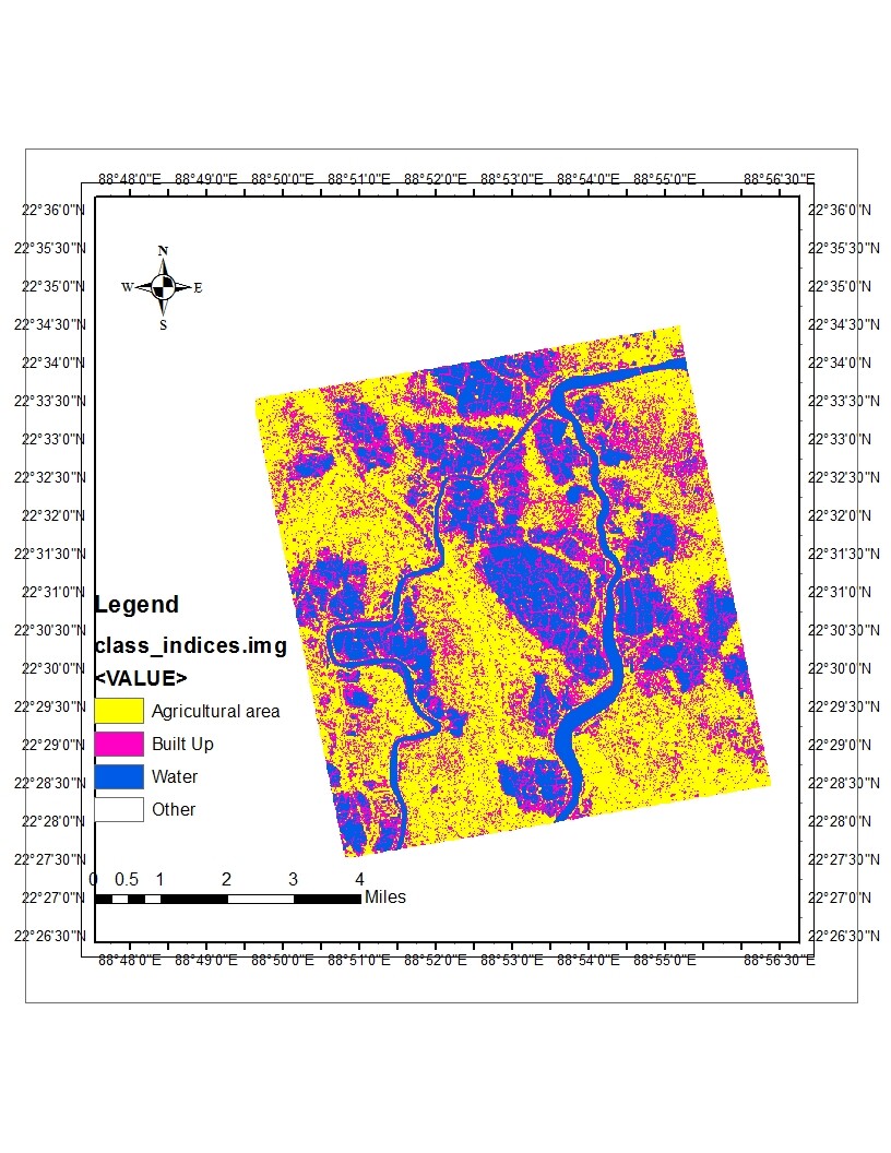
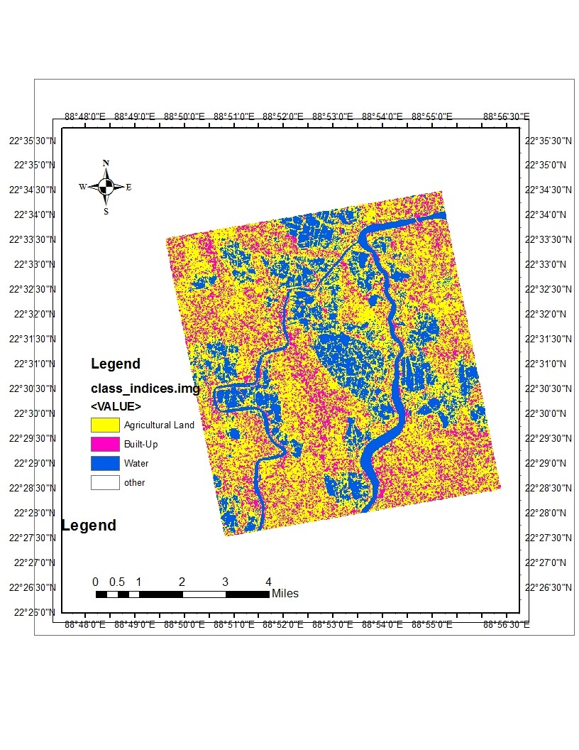
But hoe can i compare these results In Snap that which one is better?
this depends on how you define “better”.
SNAP has no tool to measure the compactness or fractality of classes. But you could digitize validation polygons and perform an accuracy assessmet as suggested in this tutorial: Landcover classification with Sentinel-1 GRD
“As highlighted by the histograms in Figure 9, the values of Sigma0_VV roughly range between 0 and 1,
with average backscatter values of 0.07 (VV) and 0.02 (VH).”
This tutorial mentions this thing. How did you calculate the average backscatter of VV and VH band on the whole?
Thanks @ABraun its a great tutorial . I learnt many new things while reading it.
In this you have used rule based classification to assign values. for different land-cover classes.
Using pixel manager first the different land cover were known at the first.
eg I make a table taking the pixel value and the corresponding backscatter value.
We can use the classification tree model to separate the classes. Which tool will help me implement something like this?
You can do this with the statistics too ![]() . It works for entire bands or pixels under selected vectors
. It works for entire bands or pixels under selected vectors
When you export pixels of your training data as a table where one column contains the class name and the other columns contain the pixel values of your raster bands, you can train a classification three which gives you thresholds. This can be done in Orange, for example: https://www.youtube.com/watch?v=D6zd7m2aYqU