Hi, during the last few weeks I experimented a little bit with StaMPS and some COSMO-SkyMed data I have access to. Unfortunately, as I explain in the end, the result does not look very satisfactory for the moment. I will keep doing some experiments, but if in the meantime more experienced people are willing to help me, they’ll have my gratitude!
Having access to a copy of SARscape, I have run the same data with it, obtaining a much better result. Therefore I believe the data is fine. On the other hand I know people are routinely use StaMPS to obtain very good data, so the problem is clearly in how I am using it, not in the program itself.
Hopefully this can also be useful for other newcomers who want to do PSI processing with CSK. Although, admittedly, a tutorial saying that it doesn’t work is not that much worthy. Let me also notice that my aim with this analysis is to capture movements of single buildings (with respect to buildings around), in order to assess potential structural problems. So I am interested in the movements of single PSs, or localized clusters of PSs. I understand this is not the aim StaMPS was written for, but for the moment StaMPS is the only free software solution I know of.
The data
I am working with 52 SLC images taken by CSK between January 2012 and December 2014, for a total of 3 years, of the area surrounding Venice, Italy. Images are polarized HH, taken on the same descending orbit, looking on the right, in Stripmap HIMAGE mode. All images are taken by the same satellite, CSKS1. More technically, all processed files have name starting with CSKS1_SCS_B_HI_01_HH_RD_SF, according to the CSK conventions.
Stack creation with SNAP
I am using SNAP through its command line processor gpt. The graph I am using are inspired by snap2stamps, which I cannot use directly because they are targeted at Sentinel-1 data.
-
Subsetting: first step is to subset the huge CSK data to a small rectangle just enclosing the main island of Venice, without subsampling.
-
Coregistration: Each image is coregistered with respect to the master image (which is taken in 2013/09/03, and was selected by mean of SNAP’s stack overview tool). Thus I create N-1 stacks, each of which with two images (the master and one slave). I know I could also create one stack with all the images at once, but I guess the coregistration result shouldn’t change, right? Coregistration parameters are the default from SNAP, and they seem to work well.
-
Interferogram generation: From each two-images stack the interferogram is computed, subtracting both flat Earth and topografic contributions. I am using SRTM 1sec HGT as DEM, with the other options set to SNAP’s default.
Looking at the interferograms, I see that those who have a small spatial baseline (no more than 100 meters) are quite good, even if the time baseline is more than a year. On the other hand, when the spatial baseline is larger, the city is barely recognizable. I guess that’s pretty normal, and that StaMPS should be able to extract useful data even from images where I can’t see anything, right? See two example images here.
-
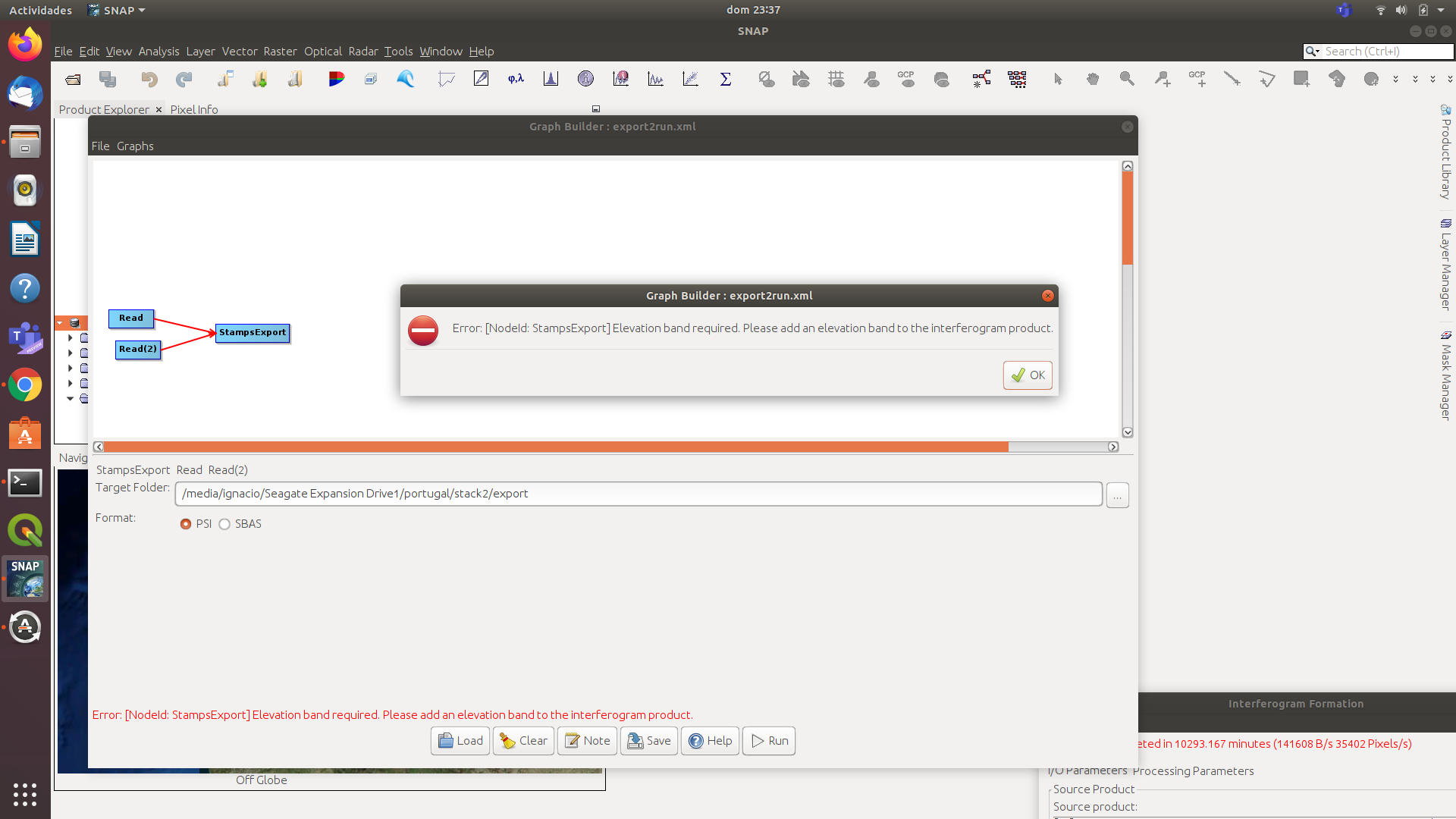
Exportation to StaMPS: this step is pretty standard and has basically no settings.
StaMPS processing
StaMPS preparation is done using 0.4 as initial threshold for amplitude dispersion. Then the following commands are given to change the StaMPS default values:
setparm('max_topo_err', 10);
setparm('filter_grid_size', 40);
setparm('clap_win', 16);
setparm('scla_deramp', 'y');
setparm('percent_rand', 1);
setparm('unwrap_grid_size', 50);
setparm('unwrap_time_win', 180);
setparm('scn_time_win', 180);
setparm('scn_wavelength', 50);
setparm('unwrap_gold_n_win', 16);
I took these default values from this tutorial, figuring out that the case “bridge” is the most similar to my study. Then I just run steps 1 through 8. I am not using TRAIN, because I haven’t really figured yet how to install it, although my understanding is that the troposferic component isn’t really important when one wants to study (relatively) small objects like single buildings.
Visualization with StaMPS_Visualizer
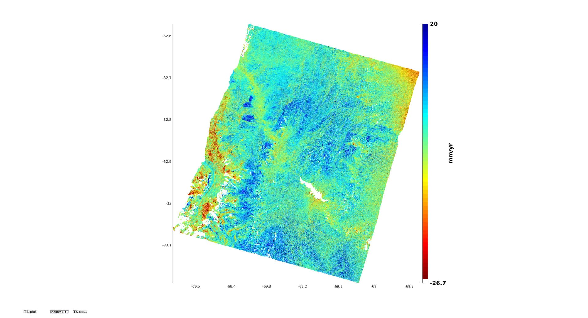
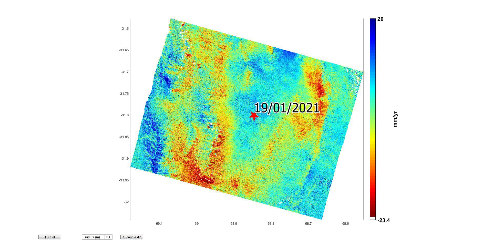
Esportation to the StaMPS_Visualizer is done with the MatLab script provided by the author, except that I am using ps_plot('v-do') instead of v-doa (because I don’t have atmospheric correction data from TRAIN). Also, I am producing two different visualizations; one, that I dub “spot”, is what the exportation script produce: all the points around a user-selected center point, within a certain radius. The other one, called “decimated”, considers the whole analyzed area, but randomly takes just one point every ten to avoid overloading StaMPS_Visualizer.
The result is available here (sometimes it doesn’t work properly with Firefox; Chrome/Chromium seems to work better). The same viewer also shows the analysis generated by SARscape (a commercial, proprietary software for SAR analysis I happen to have access right now) on the same data.
Why I am not very satisfied with StaMPS?
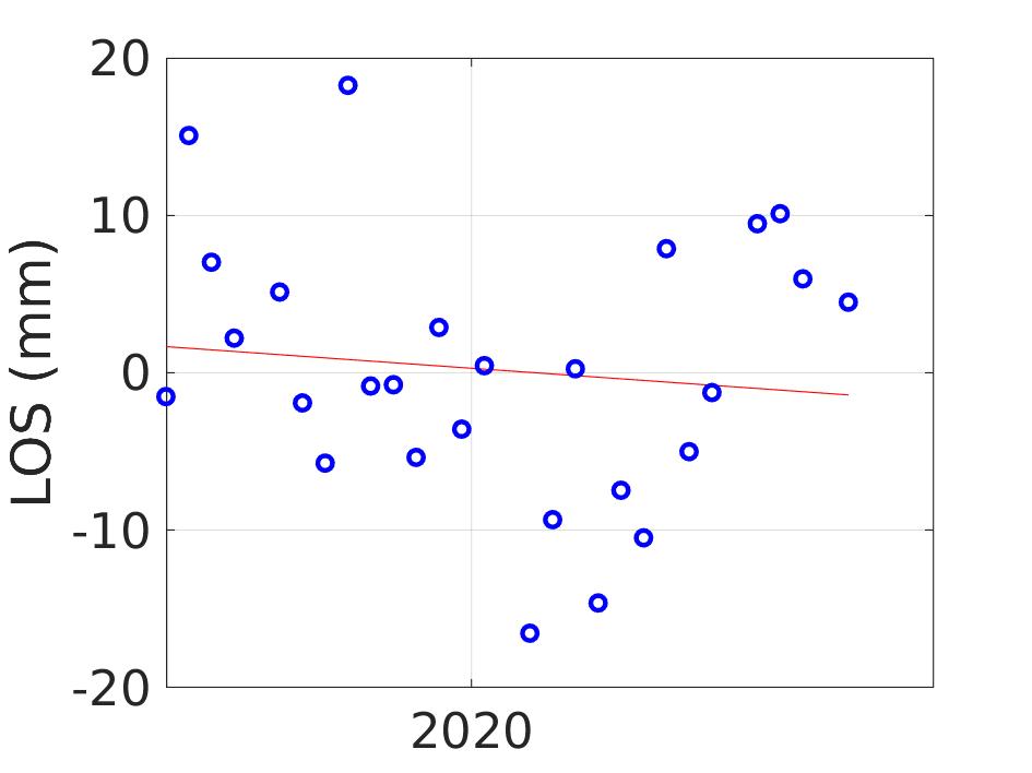
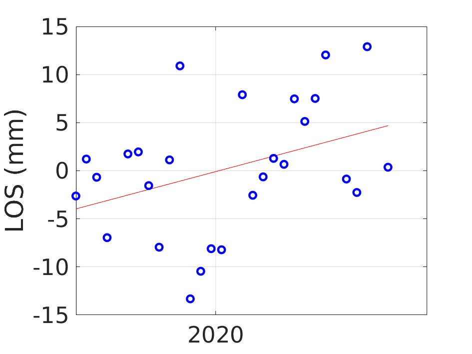
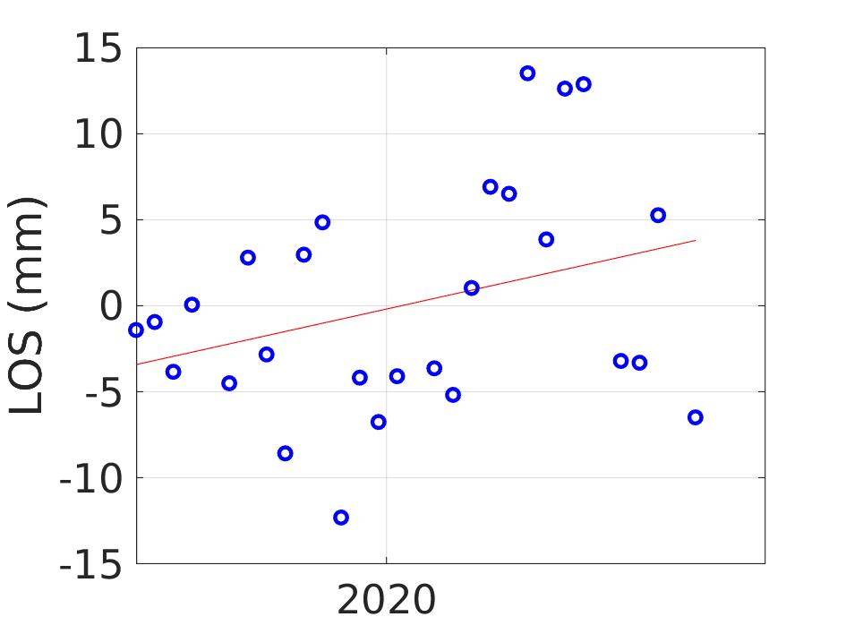
Unfortunately the history of the PSs generated by StaMPS analysis often seem to be very noisy, especially comparing with SARscape results. If you go on the visualizer and click a random dot for a StaMPS analysis, you will probably see jumps of 10-15 mm around the linear regression, while SARscape points jump around 1-3 mm around the linear regression.
Beside the relative comparison, 15 mm is half the wavelength of COSMO-SkyMed X band SAR instrument. This means that it is very probably that the phase unwrapper got completely confused by this data and there is very little trust that the average unwrapped trend actually matches the linear displacement trend of the scatterer.
What do you think?
I am very newbie to this field; I am still learning a lot of things and no doubts I might have done mistakes in the analysis or fed wrong parameters to SNAP or StaMPS. Do you agree with the reasons I believe that data computed by StaMPS is not good in my case? What would you suggest to fix it?
Thanks for reading such a long post if you got there, and even more thanks if you have useful advice to spare!