I started to work with S-2 MAJA processed data.
My workflow:
Bands extractor to only keep 10 bands (Flat reflectance) + cloud mask
Resampling the 20m bands
Reprojecting to local CRS
I would like to export the result as geotif but all the bands in seperate files.
So it is somehow like the MUSCATE original format.
So far I have not figured out how to do this. Export Geotif only produces mulitlayer raster.
Thanks for the help
when you have taken the WKT from the reprojected scene then it is okay to do the subsetting after the reprojection.
It should also be fine if you take the WKT from the original S2 scene, which is in UTM CRS. Then doing the subsetting first and then the reprojection. Sure, both will lead to different results but should be -somehow- in line with the original polygon.
In both cases the subsetting is using the bounding box of the polygon.
Right now, I can hardly imagine what the difference between the processing result and the expected polygon is. Can you provide some images?
In terms of performance, it doesn’t matter much in which order you do the subsetting. Because it is only processed what is written to the output. Doing the subsetting first might be a bit faster.
To me, “data cube” is just a 3-D array. Older software may only support GeoTIFF, some newer software won’t make a data cube from heterogeneous 2-D images because the metadata support assumes consistent scaling, units, etc. for all cells. Newer software may call a heterogeneous data cube a “stack” and preserve metadata for each layer.
Many use the subsetting on S2 data and they are happy with the results. So, in general it works quite well.
You could try to create the polygon in SNAP or describe your process in more detail. Share the polygon and mention the name of the product you are using. Maybe there is a mittle mistake somewhere.
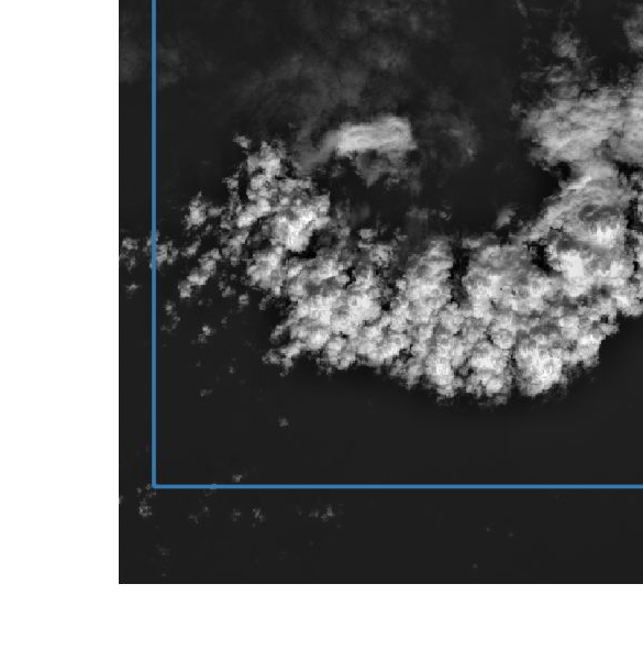
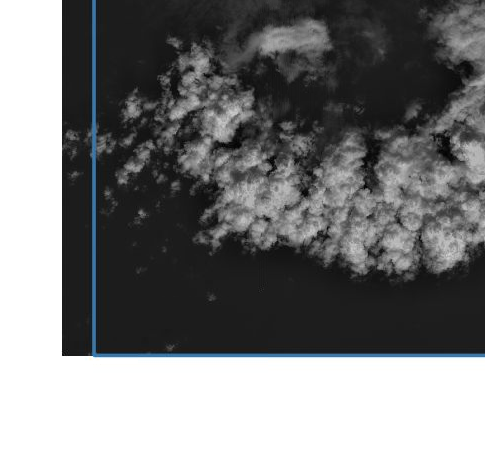
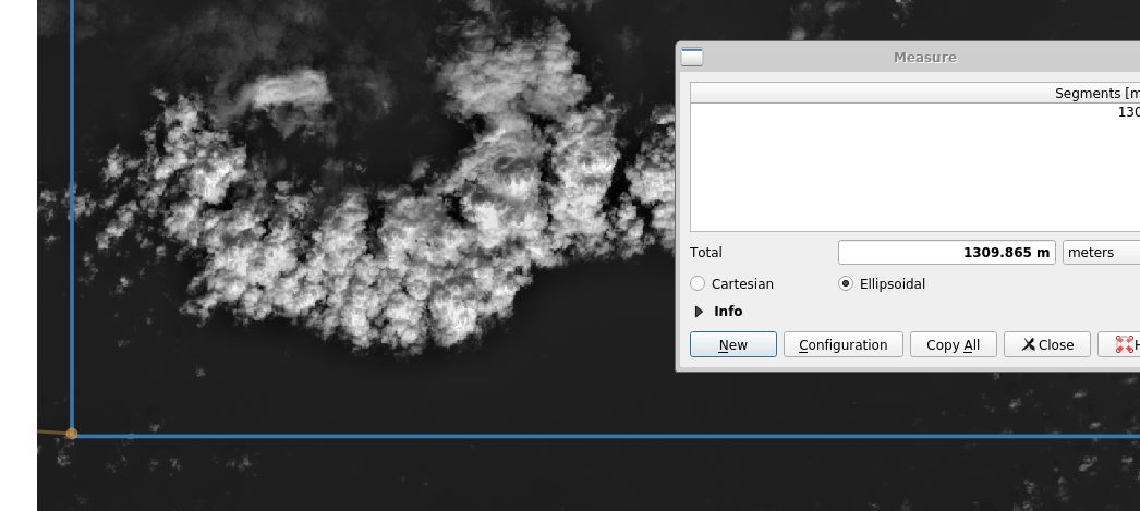
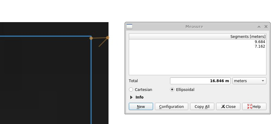
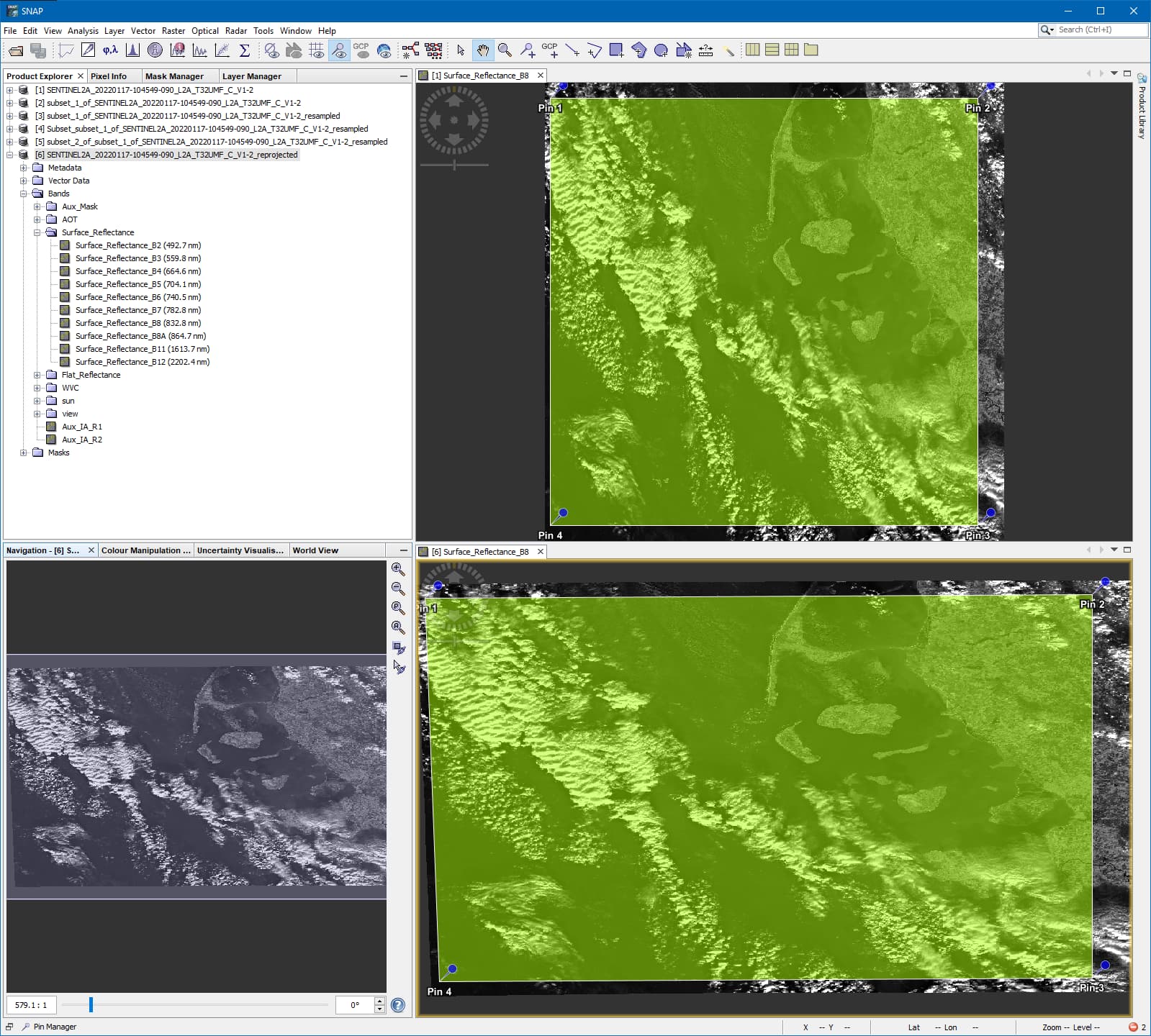
At the top you see the original MAYA processed image with the polygon and pins at the corners.
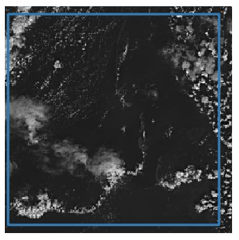
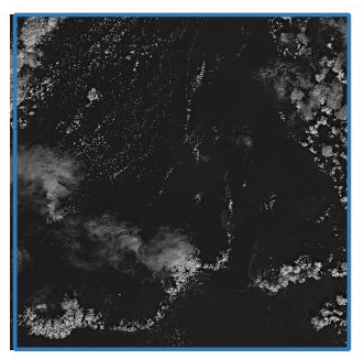
At the bottom you see the same image reprojected to WGS84.
You can notice the distortion of the polygon mainly on the left. And this causes the differences.
The coordinates for the subset are given in WGS84 space.
From the transformed shape the bounding box is used and then the subset is created.
The creates the difference you observe. So, in WGS84 terms the subset calculation is correct.
But not what a user expects.
this is very interesting.
To get a better understanding…
…if I open a MAJA original product in SNAP, it comes projected in EPSG:32 632 from DLR,
does SNAP get this information about the projection from the metadata-file?
Or does the Software assume every opened product is in EPSG:4326?
What would be a smart workaround?
To transform all the 7 polygons in QGIS into EPSG:4326.
Load the MAJA product and also transform it into EPSG:4326
Do the substet and transform it again into the EPSG:25832, what is the preferd CRS for the final product?
It sounds like lots of transformations.
Can you think of anything smater?
Regards Christian
You could look up the corner coordinates in pixel of the non-overlapping pixel for the tiles. Using the pixel-coordinates the subset should work.
If the tile is not at a UTM zone border the coordinates are constant for all tiles.
The overlap is 10Km. So, in 10m resolution you need step into the 1000pixels. For 20m resolution 500 pixels.
At UTM borders you need to look up the coordinates. Here the coordinates can vary.
Hi Marco, it took me a while to figure out the exact pixel position to do the subset for all seven tiles. But in the end it seems to work =) . The result from SNAP is the same as the cliped subset from QGIS. Thanks for the support.
Another thing came to my attention.
A safed graph with resampling does not keep the information.
So when bulk processing is started the CRS has always be changed again (in my case EPSG25832).
If forgotten the transformation is not correct as SNAP uses WGS84.
Is there a reason why individual changes are not kept during saving?
I’m not often using the Graph Processor and the Bulk Processing. I usually use the command line.
In general, the parameter should be saved with the graph.
Maybe @ABraun or @lveci have an idea what’s going wrong.
Hi guys…a little different topic but still the same project. So I keep it in this discussion rather than opening a new one.
I saved my processed data.
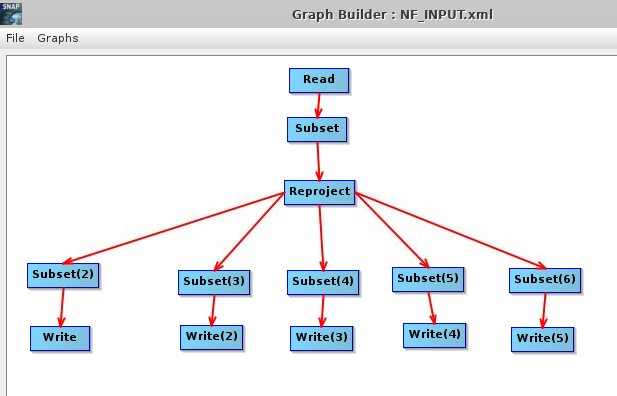
Graph looks as follows:
so
Subset bands (at the moment I will only use the 10 m bands and a cloud mask)
Reprojection from EPSG32632 to EPSG25832…
Subset to seperate the bands and clip to pixel extend
write the product as gtiff
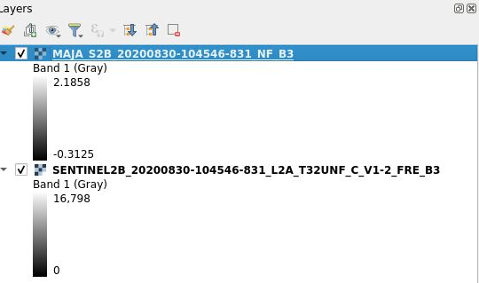
Now if I open the processed product and the raw data from DLR I get a significant difference in the grey-value-range.
The original MAJA product is surface reflectance x 10000. so the raw product with a range from 0-16798 seem okay.
But my processed product from SNAP with -0,3125 - 2,1858 seems akward…
Do I missunderstand something…maybe someone with a litte more experience can clear this up a little…would be greatful for some input.
Cheers
Christian
For me it seems that these are the scaled values.
In the Geotiffs you have created, the actual reflectance values are stored and not the raw values.
Does the value range fit to the Maya data when you open it in SNAP?
I did some testing with the data.
Reason for the difference seems to be the MUSCATE importer in SNAP.
(see pdf - the created geotiffs and the raw data imported via the MUSCATE-importer have same value range…same as in QGIS)
This is the reason why values are changing.
But still I can´t see why it is shifting the reflectance into negative values.
Is there any documentation what the MUSCATE importer is doing and why the overall range is changeing? The product description from MAJA only tells me that the values are surface reflectance multiplied by 10000.