Hi @ABraun, sorry for late update  I am here again to share my new results.
First of all… since I noticed in order to generate a DEM, I made the following mistakes:
-
I used wrong steps with incorrect parameters.
-
My original target area is not suitable for making a DEM since there are too many mountainous area involved. Besides, this area is one of the most rainy area in Taiwan, which means the humidity here is quite high. I think these factors all play important roles in low coherence value in the end.
-
The perpendicular baseline I used in the original images are only 0.01 m which is so ridiculously low… orz
So, I made a new try here. 
The following are my steps according to how I choose my new target area, SAR images and steps I used to generate DEMs:
Firstly, I choose mid-Taiwan as my target area since here is relatively dry in comparison to other areas in Taiwan.
Secondly, I choose SAR images of winter time because the weather is drier and less rainy. In addition, plants don’t grow during winter so I assume more bare area can lead to higher coherence value.
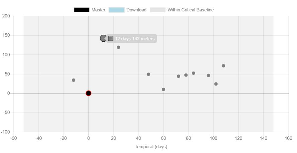
Thirdly, based on the information I have learned from the forum, I checked if there are any SAR img pair available with 150~300 m of perpendicular baseline by the website UAF, https://baseline.asf.alaska.edu/#/baseline. However, the maximum baseline I could find is 141 m with 12 days of temporal gap which I think is acceptable.
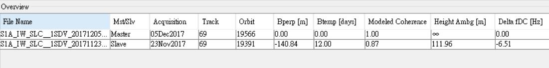
Fourthly, I downloaded this two Sentinel-1A SLC products.
By the way, I also checked that this two days were not raining on 2017.11.23 and 2017.12.05, but the relative humidity is range from 62~69%. (it is still a bit too high I think…)
Fifthly, I generate DEM by the following steps: (bold fonts means the process that I did incorrectly before.)
-
S-1 TOPS Coregistration
-
Interferogram Formation (without topographic phase removal)
-
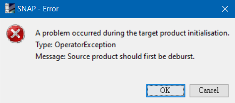
S-1 TOPS Deburst
-
Goldstein Phase Filtering
-
Snaphu Export (choosing TOPO as my statistical-cost mode and MCF as my initial method)
-
Run unwrapping using Cygwin
-
Snaphu Import
-
Phase to Elevation
-
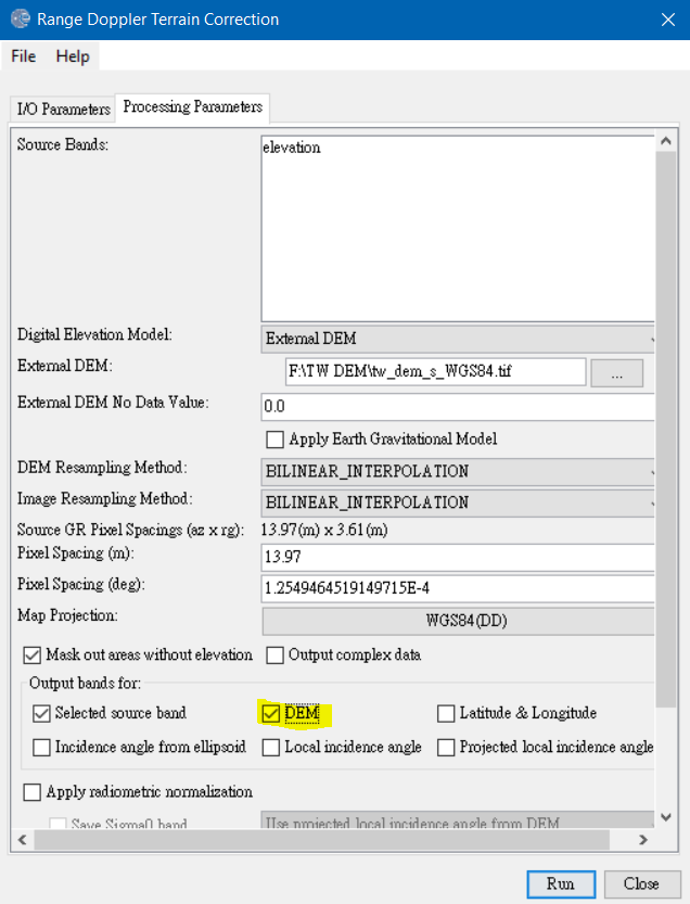
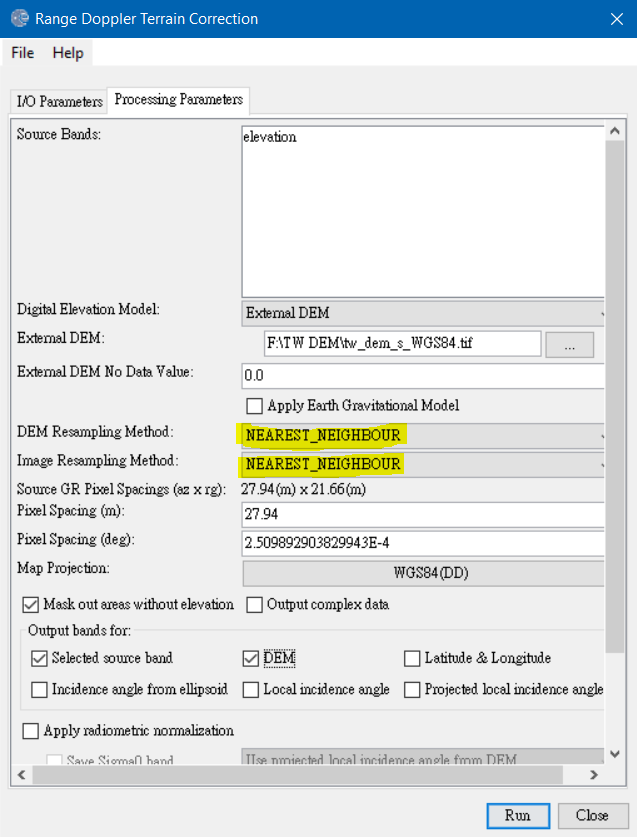
Range-Doppler Terrain Correction
OK…Finally!
Now here comes my test design and my comparisons:
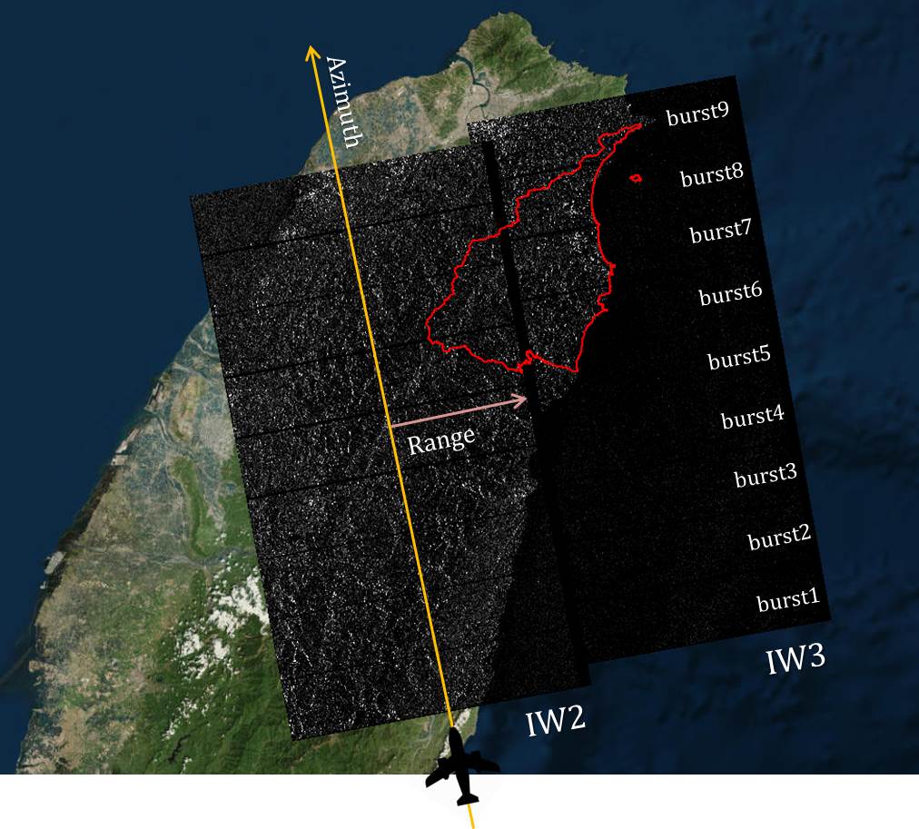
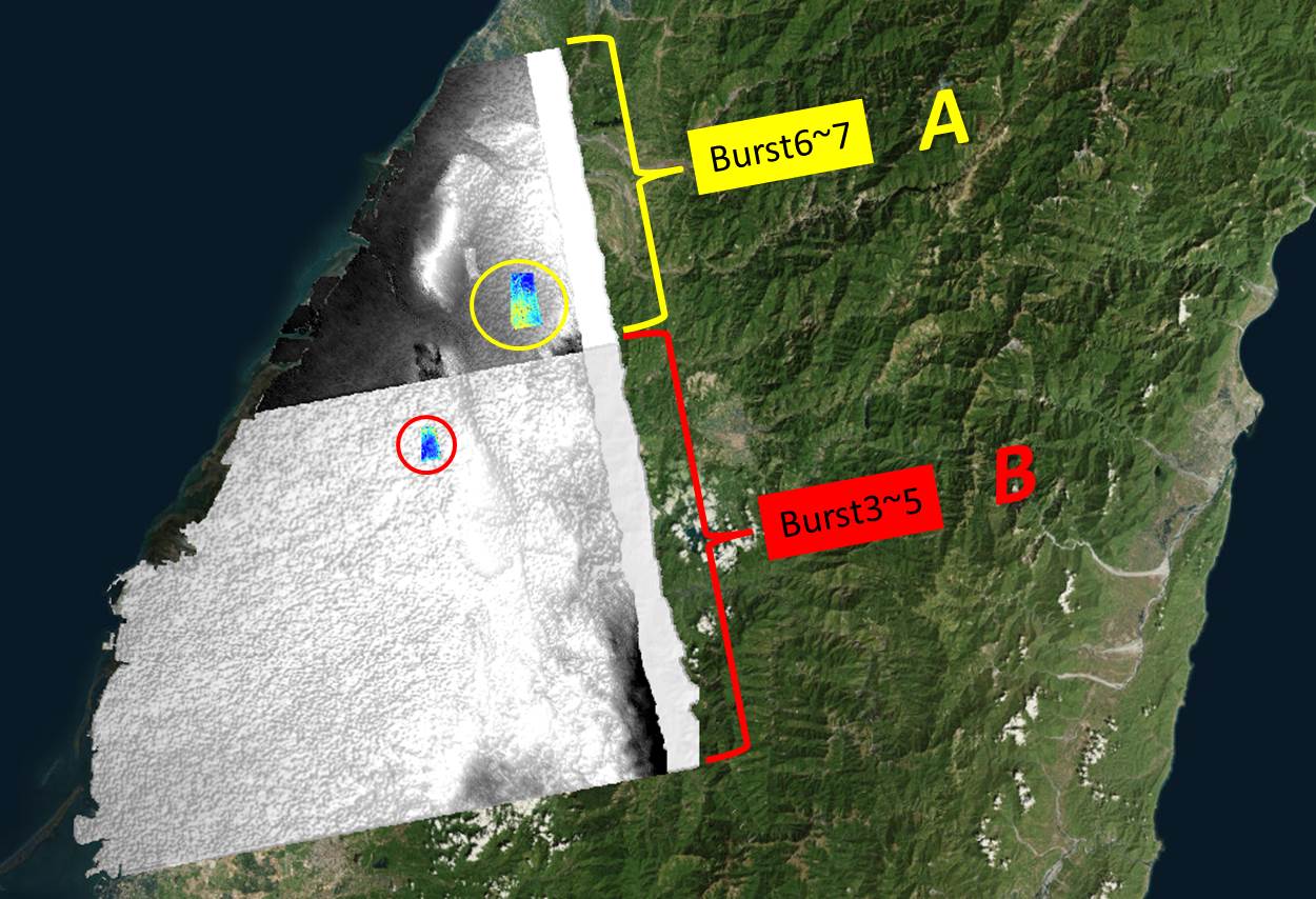
I have two test areas here which are called A (using swath 1 and burst 6~7) and B (using swath 1 and burst 3~5). A has a higher coherence value in general since here involves more urban area.
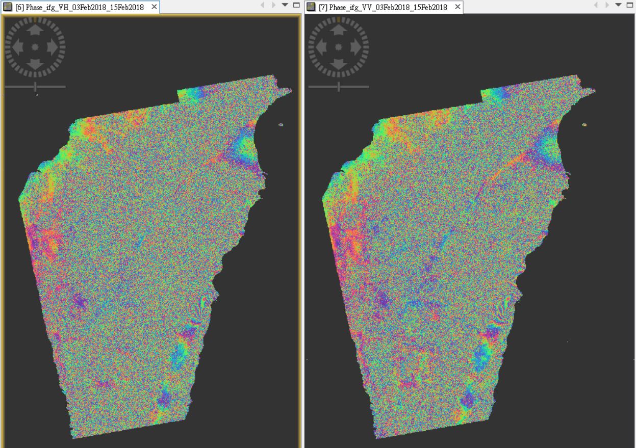
In each area, I generated DEM with both VV and VH polarization in order to see different result with different polarization.
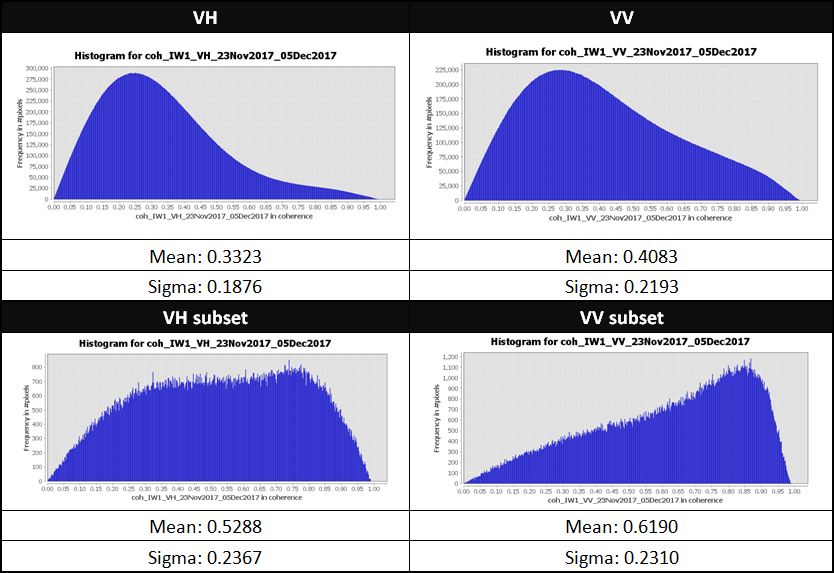
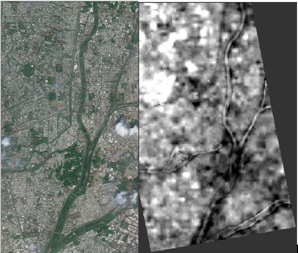
Then, I select a subset area base on stronger intensity shown in the output file after coregistration, and operate the same process again to see if a stronger coherence value will lead to better result. The subset areas are indicated as yellow and red circles in the figure.
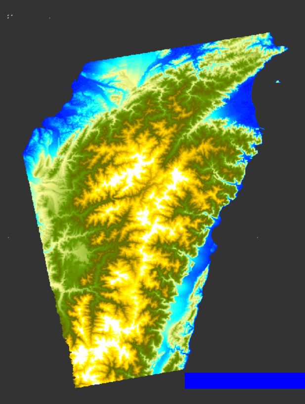
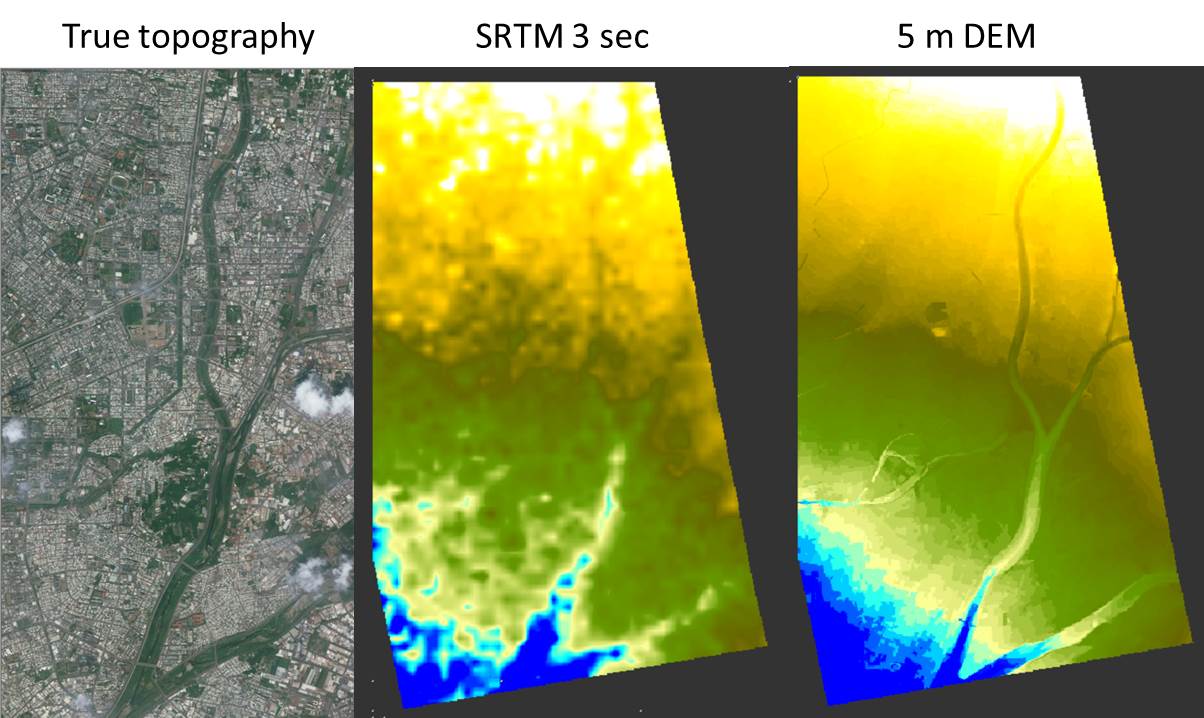
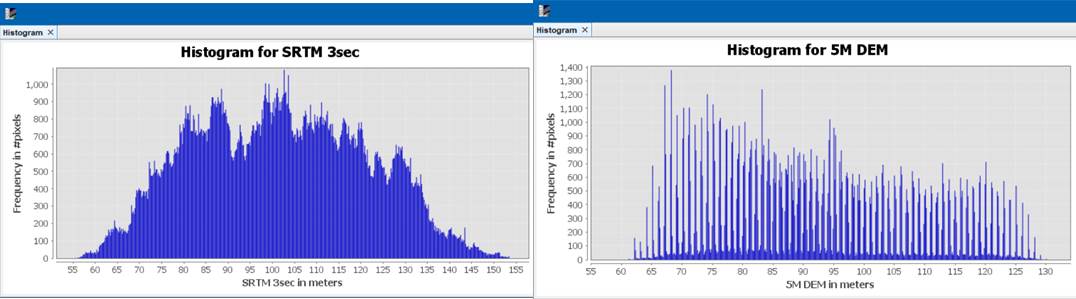
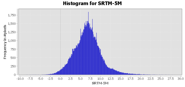
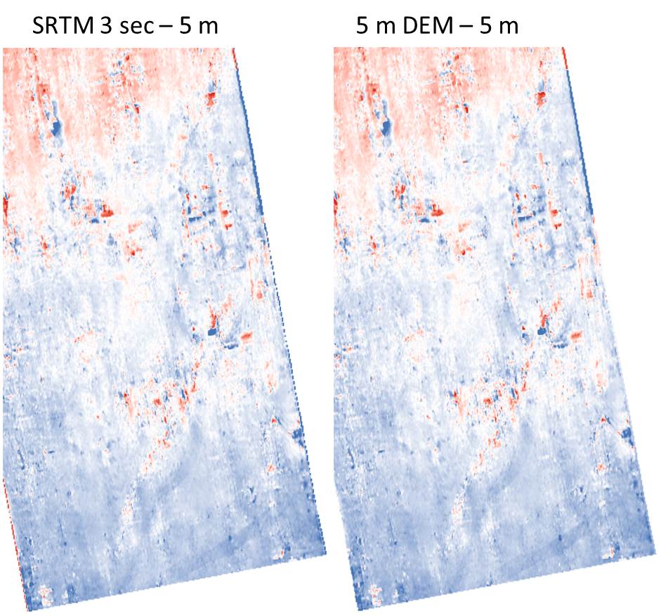
I import the DEMs into GIS and compare to my 5 meter DEM (as true value), and I notice that the coherence value REALLY has a strong influence on the accuracy of output DEM!
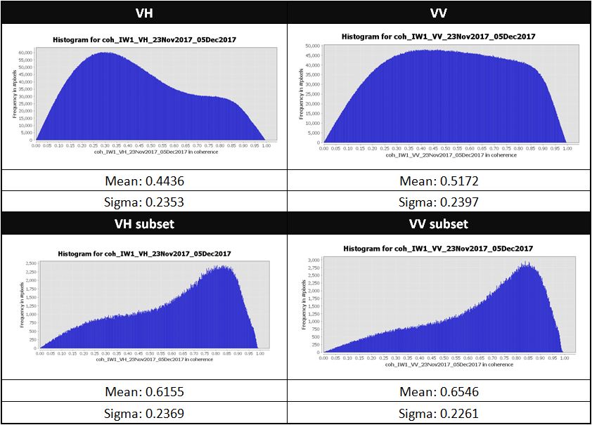
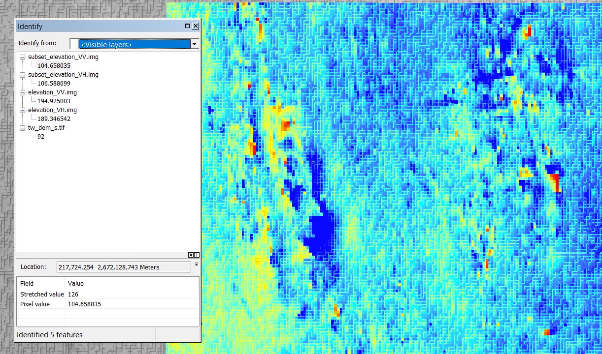
Let’s see the coherence value of B area first. After comparison, I notice that:
-
The coherence value of VV is about 0.1 better than VH, however, it does not necessary reflect to the accuracy of dem. For example, before subset, VH performs 6 meters better then VV but after subset, VV performs 2 meters better than VH.
-
Subset areas perform considerably better. Before subset, the error is at least 100 m, but it improves up to under 15 meter after subset!
P.S
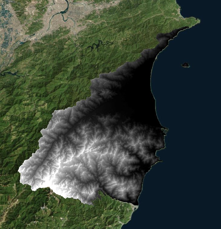
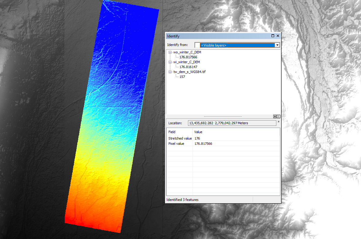
tw_dem_s is my 5 m dem, which is seem as true value here.
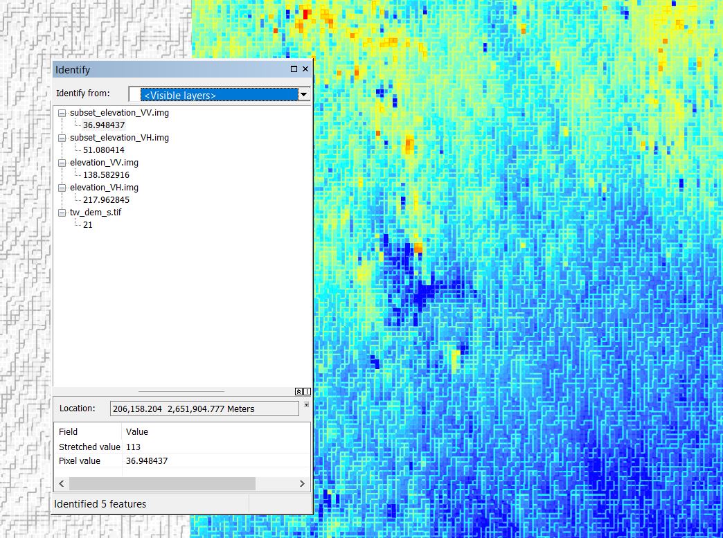
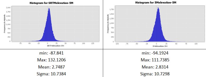
Now let’s see the coherence value of A area. The discover is the same as what we have learned from area B, but still we can make the following remark:
- The coherence value of area A improves 0.1 than area B which leads to a higher accuracy in output DEMs. This can be proved by the error between two area pairs. Without subset, errors in A can be limited to 100 m. With subset, errors in A can be limited to 10 m.
P.S
tw_dem_s is my 5 m dem, which is seem as true value here.
The above is my test. I know simply click several points in GIS is not the best way to see the general trend and conduct my comparisons and so on, however, since I only want to make it an easy try, I don’t want to make a sophisticated statistic computation in GIS (using raster calculation or so).
Ok, here I have several questions:
-
Even if I have already tried whatever I have thought about to increase my coherence value, the best result here only shows roughly 10 meters accuracy. I wonder if I can make any more improvements to improve the quality of my DEM?
-
My DEM, as shown in the above images, are somehow “gridish” which means the value is not continuous. I wonder if it is normal or did I make anything wrong?
Thanks for reading and I am really grateful to any of your reply! If you find any incorrect part or you have any suggestion, please feel free to offer me your valuable comments