StaMPS-Visualizer, SNAP-StaMPS Workflow

[thho]

@suribabu this error was reported and solved several times already. The solution is also documented in the Manual tab within the app. Go StaMPS-Visualizer --> Manual --> Troubleshooting you find

…sometimes an error occurs like horzcat matrix is not consist with each other. to avoid this error, make a new ts plot and select a very large search radius which includes all MP…

use a large radius for the ts plot like 1000000

please do as @ABraun mentioned earlier

Surface Subsidence

and avoid cross posting to keep this board as structured as possible.

[suribabu]

Thank you so much Thho and ABraun.

[suribabu]

I followed all the steps in the Stamps manual, Above one is the stamps(6,6) output after rerun shown in above stamps manual.
(ps_plot(‘u’)).

Then i ran stamps(7,7) below one is the output,

stamps(7,7)

STAMPS: ########################################
STAMPS: ####### StaMPS/MTI Version 4.0b6 #######
STAMPS: ####### Beta version, Jun 2018 #######
STAMPS: ########################################

STAMPS: Will process current directory only

STAMPS: ########################################
STAMPS: ################ Step 7 ################
STAMPS: ########################################
STAMPS: Directory is 6_psiexport

PS_CALC_SCLA: Starting
PS_CALC_SCLA: Estimating spatially-correlated look angle error…
GETPARM: small_baseline_flag=‘n’
GETPARM: drop_ifg_index=
GETPARM: scla_method=‘L2’
GETPARM: scla_deramp=‘y’
GETPARM: subtr_tropo=‘n’
GETPARM: tropo_method=‘a_l’
GETPARM: scla_drop_index=

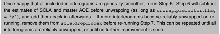
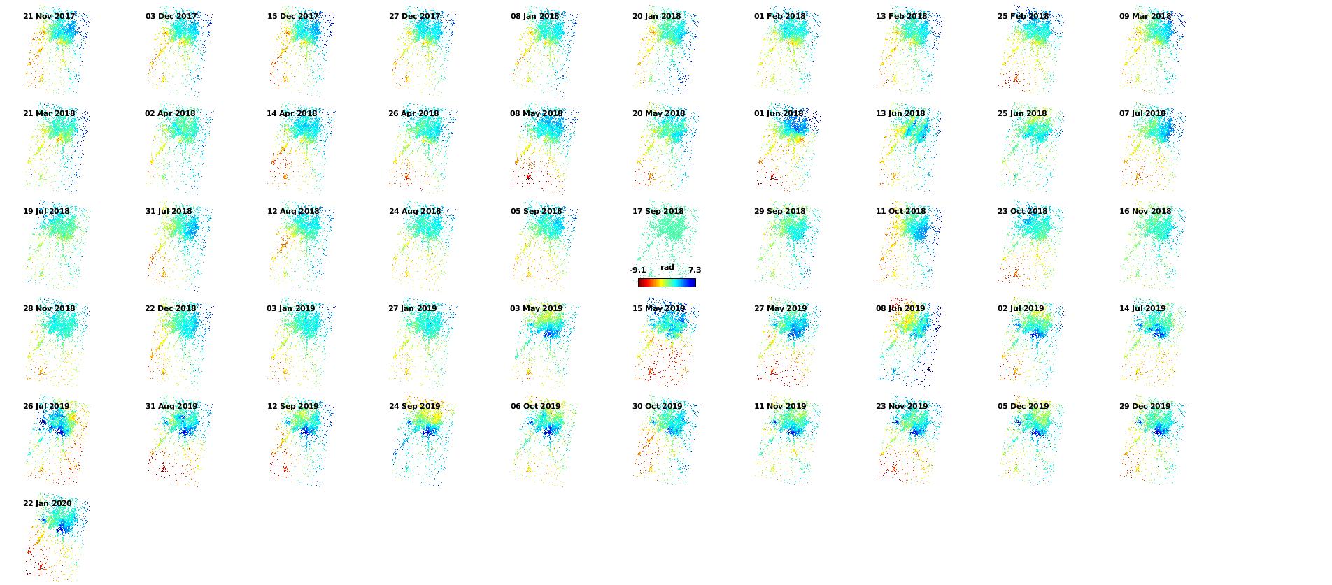
deramping ifgs…
Deramping computed on the fly.
**** z = ax + by+ c
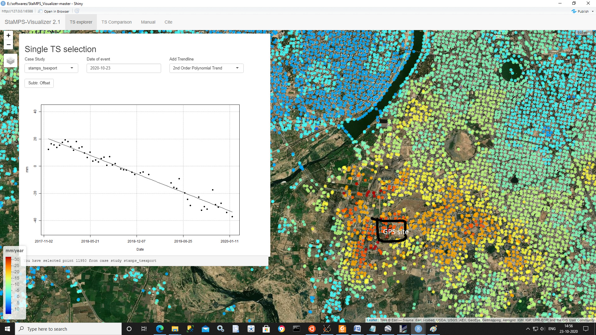
44182 ref PS selected
PS_CALC_SCLA: 50 ifgs used in estimation:
PS_CALC_SCLA: 21-Nov-2017 to 03-Dec-2017 12 days -59 m
PS_CALC_SCLA: 03-Dec-2017 to 15-Dec-2017 12 days 0 m
PS_CALC_SCLA: 15-Dec-2017 to 27-Dec-2017 12 days -63 m
PS_CALC_SCLA: 27-Dec-2017 to 08-Jan-2018 12 days 58 m
PS_CALC_SCLA: 08-Jan-2018 to 20-Jan-2018 12 days 74 m
PS_CALC_SCLA: 20-Jan-2018 to 01-Feb-2018 12 days -27 m
PS_CALC_SCLA: 01-Feb-2018 to 13-Feb-2018 12 days 24 m
PS_CALC_SCLA: 13-Feb-2018 to 25-Feb-2018 12 days -77 m
PS_CALC_SCLA: 25-Feb-2018 to 09-Mar-2018 12 days -46 m
PS_CALC_SCLA: 09-Mar-2018 to 21-Mar-2018 12 days 42 m
PS_CALC_SCLA: 21-Mar-2018 to 02-Apr-2018 12 days 75 m
PS_CALC_SCLA: 02-Apr-2018 to 14-Apr-2018 12 days 1 m
PS_CALC_SCLA: 14-Apr-2018 to 26-Apr-2018 12 days -30 m
PS_CALC_SCLA: 26-Apr-2018 to 08-May-2018 12 days 1 m
PS_CALC_SCLA: 08-May-2018 to 20-May-2018 12 days -9 m
PS_CALC_SCLA: 20-May-2018 to 01-Jun-2018 12 days -52 m
PS_CALC_SCLA: 01-Jun-2018 to 13-Jun-2018 12 days 118 m
PS_CALC_SCLA: 13-Jun-2018 to 25-Jun-2018 12 days -36 m
PS_CALC_SCLA: 25-Jun-2018 to 07-Jul-2018 12 days -93 m
PS_CALC_SCLA: 07-Jul-2018 to 19-Jul-2018 12 days 53 m
PS_CALC_SCLA: 19-Jul-2018 to 31-Jul-2018 12 days -31 m
PS_CALC_SCLA: 31-Jul-2018 to 12-Aug-2018 12 days 61 m
PS_CALC_SCLA: 12-Aug-2018 to 24-Aug-2018 12 days -37 m
PS_CALC_SCLA: 24-Aug-2018 to 05-Sep-2018 12 days 84 m
PS_CALC_SCLA: 05-Sep-2018 to 17-Sep-2018 12 days -57 m
PS_CALC_SCLA: 17-Sep-2018 to 29-Sep-2018 12 days -14 m
PS_CALC_SCLA: 29-Sep-2018 to 11-Oct-2018 12 days 23 m
PS_CALC_SCLA: 11-Oct-2018 to 23-Oct-2018 12 days -25 m
PS_CALC_SCLA: 23-Oct-2018 to 16-Nov-2018 24 days 3 m
PS_CALC_SCLA: 16-Nov-2018 to 28-Nov-2018 12 days -36 m
PS_CALC_SCLA: 28-Nov-2018 to 22-Dec-2018 24 days 48 m
PS_CALC_SCLA: 22-Dec-2018 to 03-Jan-2019 12 days -16 m
PS_CALC_SCLA: 03-Jan-2019 to 27-Jan-2019 24 days 37 m
PS_CALC_SCLA: 27-Jan-2019 to 03-May-2019 96 days 92 m
PS_CALC_SCLA: 03-May-2019 to 15-May-2019 12 days -99 m
PS_CALC_SCLA: 15-May-2019 to 27-May-2019 12 days 16 m
PS_CALC_SCLA: 27-May-2019 to 08-Jun-2019 12 days -68 m
PS_CALC_SCLA: 08-Jun-2019 to 02-Jul-2019 24 days 82 m
PS_CALC_SCLA: 02-Jul-2019 to 14-Jul-2019 12 days -37 m
PS_CALC_SCLA: 14-Jul-2019 to 26-Jul-2019 12 days -18 m
PS_CALC_SCLA: 26-Jul-2019 to 31-Aug-2019 36 days 20 m
PS_CALC_SCLA: 31-Aug-2019 to 12-Sep-2019 12 days -39 m
PS_CALC_SCLA: 12-Sep-2019 to 24-Sep-2019 12 days 66 m
PS_CALC_SCLA: 24-Sep-2019 to 06-Oct-2019 12 days -12 m
PS_CALC_SCLA: 06-Oct-2019 to 30-Oct-2019 24 days -35 m
PS_CALC_SCLA: 30-Oct-2019 to 11-Nov-2019 12 days 28 m
PS_CALC_SCLA: 11-Nov-2019 to 23-Nov-2019 12 days -40 m
PS_CALC_SCLA: 23-Nov-2019 to 05-Dec-2019 12 days -36 m
PS_CALC_SCLA: 05-Dec-2019 to 29-Dec-2019 24 days 107 m
PS_CALC_SCLA: 29-Dec-2019 to 22-Jan-2020 24 days -41 m
PS_CALC_SCLA: Finished
PS_SMOOTH_SCLA: Starting
PS_SMOOTH_SCLA: Smoothing spatially-correlated look angle error…
PS_SMOOTH_SCLA: Number of points per ifg: 44182
PS_SMOOTH_SCLA: Number of arcs per ifg=132514
PS_SMOOTH_SCLA: 100000 arcs processed
PS_SMOOTH_SCLA: Finished
STAMPS: Finished

Question

1. PS_CALC_SCLA: 21-Nov-2017 to 03-Dec-2017 12 days -59 m** (Is it indicating displacement from 12 days =-59m)?
2. How can i identify the bad interferograms ?

Thank you so much ABraun and thho for your continuous support to reach this steps .

[suribabu]

Below plot is the output of ps_plot(‘u-dmo’)

Thank you.

[ABraun]

@suribabu

• PS_CALC_SCLA: 21-Nov-2017 to 03-Dec-2017 12 days -59 m** (Is it indicating displacement from 12 days =-59m)?
• How can i identify the bad interferograms ?

the numbers indicate the spatially correlated look angle error. Interferograms with a large scla can be dropped testwise to see if the results become better.

[suribabu]

Dear ABraun,
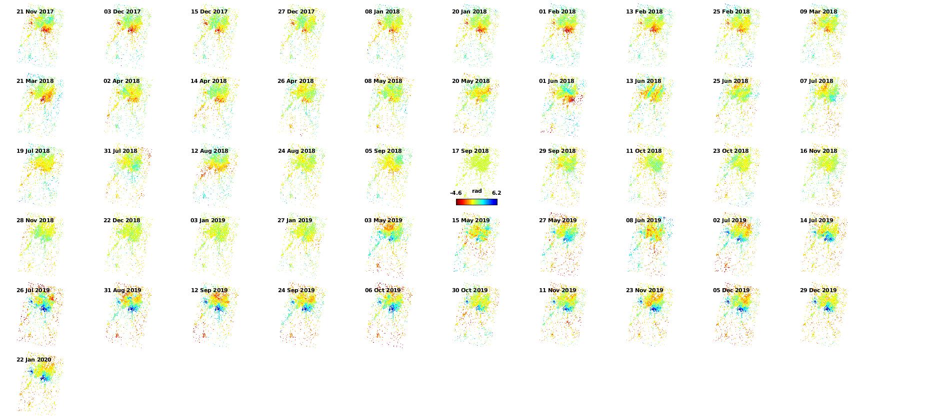
Below one is the part of my study area, wherever the subsidence happen(red colour(-10 to -24mm), in the below figure, at the same place we have a GPS station (selected in Single TS selection) running from 2 years, the time series of the GPS site also showing that subsidence at that particular area (-15mm).

Is it correct procedure to compare like this?
Thank you.

From Stamps manual:
(For plotting of velocities, the units are mm/year with positive values being towards the satellite, the sign convention for velocity was the opposite).

[ABraun]

yes, this is comparable. Two things to note when you compare the data to your GPS measurements

• StaMPS measures displacement along the line-of-sight (LOS), not directly the vertical motion.
• the time-series plot you show is the relative motion between the first and the last image in mm. The range of the y axis is quite arbitrary. It shows the temporal trend, so positive values do not mean uplift in a strict sense but that the height of this selected point is constantly decreasing.

[suribabu]

Thank you so much ABraun.
the time-series plot you show is the relative motion between the first and the last image in mm.

Up to know i though the relative motion between the master(20180917 in my study) and slave (remaining all).

[thho]

@suribabu nice result btw

[suribabu]

Thank you so much Thho…

[ABraun]

@suribabu

Up to know i though the relative motion between the master(20180917 in my study) and slave (remaining all).

yes, it was all computed against the master. Just wanted to prevent misinterpretation - good job!

[suribabu]

Dear ABraun,

While running the SNAP i used around 53 images and it’s created 52 interferograms. And the same output i used in SNAP-StamPS then it created 50 interferograms instead of 52. From where i will find these left images in StamPS.

Thank you.

[ABraun]

I don’t know what went wrong, sorry.

Maybe your master date was also included in the slaves folder?

[nachin6789]

@ABraun

Did you have a look here already?

• Phase Unwrapping to Vertical Displacement
• Horizontal and vertical displacement
• LOS Displacement vs Vertical Displacement for subsidence monitoring

They refer to traditional DInSAR approaches, so with PS you usually need results from both ascending and descending tracks and then apply some vector calculations as suggested in this paper, for example:

Hi.

I have seen several articles to discover horizontal deformation and they have seemed quite difficult to understand or replicate the process with QGIS.

Perhaps the work that has convinced me has been the following:

Vector-based approach for combining ascending and descending persistent...

However, I am still not clear about the process. That is why I would like to know if there is a manual or workflow to continue learning about insar.

Thank you very much for all the contributions

[nachin6789]

another question. how can I get standard deviation among all the analyzed points?

[ABraun]

ps_plot('vs')

[nachin6789]

Hi, nobody has an answer to this post, about if there is any manual or workflow of vertical and horizontal displacement? @ABraun @mdelgado

@nachin6789

Hi.

I have seen several articles to discover horizontal deformation and they have seemed quite difficult to understand or replicate the process with QGIS.

Perhaps the work that has convinced me has been the following:

Taylor & Francis

Vector-based approach for combining ascending and descending persistent…

(2018). Vector-based approach for combining ascending and descending persistent scatterers interferometric point measurements. Geocarto International: Vol. 33, No. 1, pp. 38-52.

However, I am still not clear about the process. That is why I would like to know if there is a manual or workflow to continue learning about insar.

Thank you very much for all the contributions

and another question @thho ;

I understand that when graphing, the displacements are cumulative movements, that is, from the first date to the second date, has moved
8,147864 mm / year and from the second date to the third date -2.5341
mm / year, etc. However, if I do the sum of all these displacements and make the average, I do NOT obtain the same average speed that is obtained from the exported Matlab file, it is very likely that I am confused, someone could explain to me what happens with the average displacement since it seems strange to me that there are variations between dates of 8.147864 mm / year, -8.443398 mm / year, etc.

[asterios_papas]

Hi there,
Hope everyone is well.

@thho @ABraun @mdelgado
I wanted to understand what exactly a time series displacement plot of a persistent scatterer from STAMPS processing truly represents.

Viewing the results of @suribabu is it wise to say that the los velocity on each specific date, is the respective value (from the .csv file) represented in the graph?

And if so, by adding all of them would you get the cumulative displacement of that specific ps, in mm, over that whole period?

Also @thho could you explain why you have added an option of subr. offset in the application? After applying it do you extract the real displacement, by providing the first date as 0 velocity and the rest is respective to it?

Sorry for the long question

Aster

[ABraun]

I think the opposite is the case: The time-series plot is the relative displacement at a point over time. It does not show the velocity over time, because that would mean that the velocity constantly decreases. In real, it shows that scatterers at this place are continuously moving away from the sensor at a (more or less) constant speed.

[asterios_papas]

@thho @mdelgado @ABraun thank you for the quick response.

That is true, if I understand correctly, it is the relative displacement based on a reference point representing close to 0 or 0 motion (seen as stable over time)?

So in stamps,if ‘ts’ displacement values of each date are provided by getting the corrected unwrapped values (step 5 to 7/8) by interferograms produces by the using same master, than each point represents the displacement of the master date and the slave date.
For example: say the first date 20171102 has a value of -17 mm and the master date is 20181207, than that value, shown in the 'ts’plot, is the displacement between those 2 dates.
Is that correct?

And if so, my main concern is if there a way to generate the cumulative displacement over time like other software ( such as sarproz etc.) produce?

I would be great to achieve such products so we could share and easily explain these products to non-eo specialist it’s already difficult to explain Los velocity results…

Hope you can help.

Aster